Tutorial Videos
This page collects Cedalion’s training videos in thirteen topics that follow a typical fNIRS/DOT analysis, from installation to reproducible pipelines. Each topic contains:
Content videos (5–15 min): slide-based lectures on concepts, theory and intuition.
Tutorial videos (5–15 min): (screen) recordings that walk through working code in Jupyter notebooks.
Example notebooks: the executable notebooks from this documentation that cover the topic. Run them locally or in the cloud via the Open in Colab button (see Running Notebooks in Google Colab).
Videos are being released step by step. Tiles marked Coming soon will link to the recording once it is published.
0. Orientation & Architecture
Start here: what Cedalion is designed for, how the toolbox is organised into subpackages, and how versioned environments and modular processing blocks keep analyses reproducible.
Content videos
0.1.C1 · Cedalion – Philosophy and Scope
0.2.C1 · Overview of Toolbox Architecture
0.3.C1 · Reproducibility & Workflows: Versioning, environments and dependency management
0.3.C2 · Reproducibility & Workflows: Functional blocks and Pipelines
Tutorial videos
Tutorial videos for this topic will show here as soon as they are recorded.
Example notebooks
No example notebook covers this topic yet.
Related documentation: Rationale · Core concepts · Environments · Changelog · All examples · Bibliography · Community
1. Installation, Execution & Data Access
How to install Cedalion locally with conda or run it on Google Colab, verify optional backends such as MCX and NIRFASTer, and download and cache the example datasets used throughout the documentation.
Content videos
1.1.C1 · Basics of Python + Installation Overview
Tutorial videos
1.1.T1 · Local installation using conda – Windows
1.1.T1 · Local installation using conda – macOS
More tutorial videos for this topic will show here as soon as they are recorded.
Example notebooks
Related documentation: Installation · Google Colab setup · Quick start
2. Data Structures & I/O
Cedalion keeps data in labelled, unit-aware xarray DataArrays that are collected in a
Recording container. This section introduces these data structures and shows how to
read and write them using the SNIRF and BIDS standards.
Content videos
2.1.C1 · Introduction to XArrays
2.2.C1 · Overview of the recording container
2.3.C1 · File formats & standards: Brief introduction to SNIRF and BIDS
2.4.C1 · Overview of Data I/O Functionality
Tutorial videos
2.3.T3 · Using the SNIRF2BIDS conversion tool
Hands-on workshop: BIDS-ifying fNIRS – a Python-based community tool for open data sharing
More tutorial videos for this topic will show here as soon as they are recorded.
Example notebooks
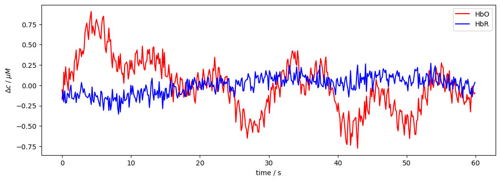
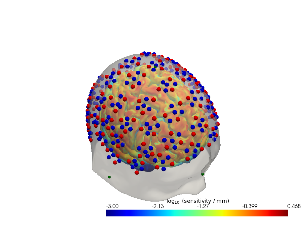
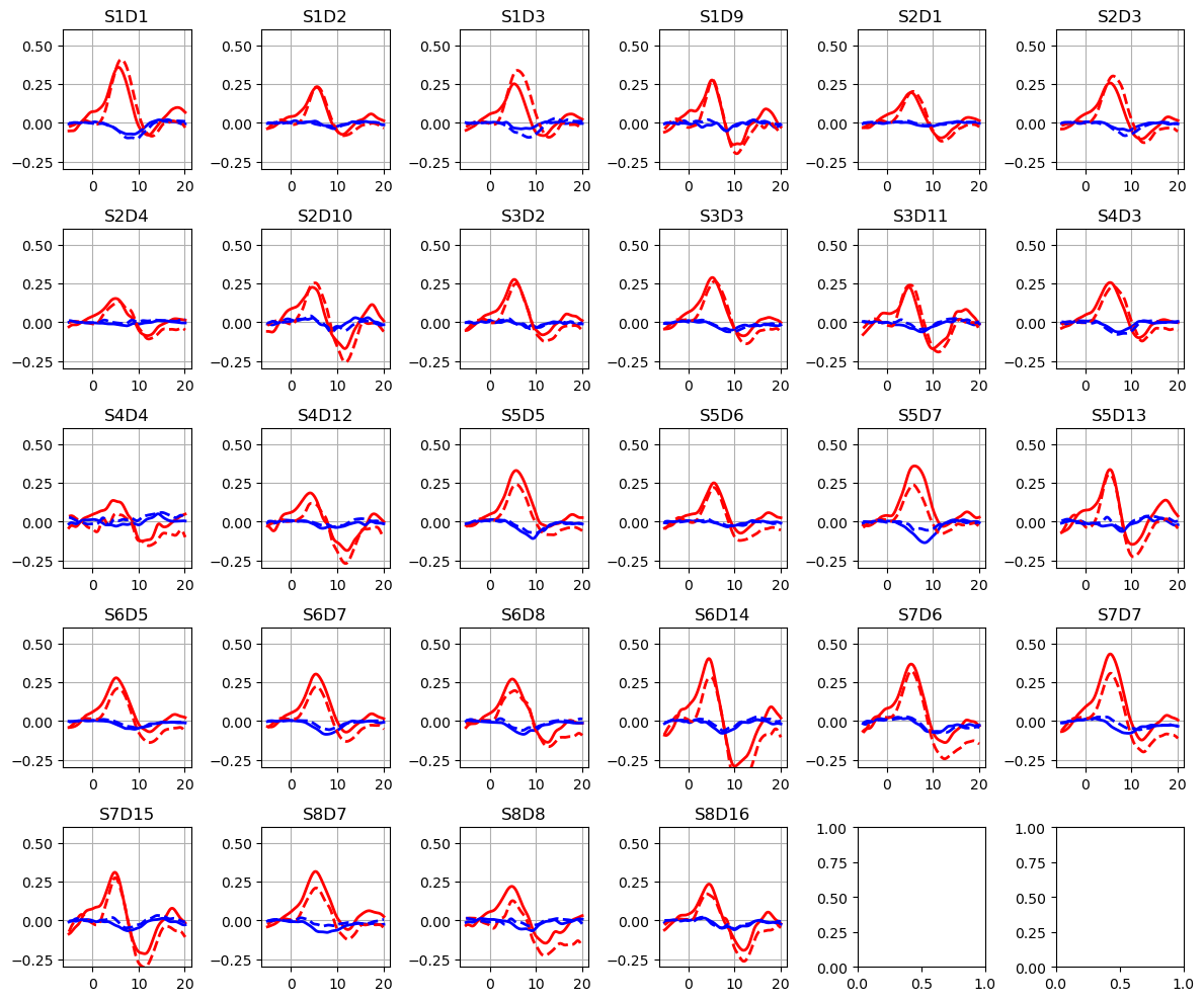
Related documentation: Data structures · Data structures and I/O
3. Modified Beer-Lambert Law
Converting raw light intensities to optical density and then to changes in oxy- and deoxyhaemoglobin concentration with the modified Beer-Lambert law, including plausibility checks and the role of source-detector distances.
Content videos
3.1.C1 · Introduction to Optical Density and the mBLL
Tutorial videos
Tutorial videos for this topic will show here as soon as they are recorded.
Example notebooks
Related documentation: Core concepts · Signal processing
4. Signal Quality & Preprocessing
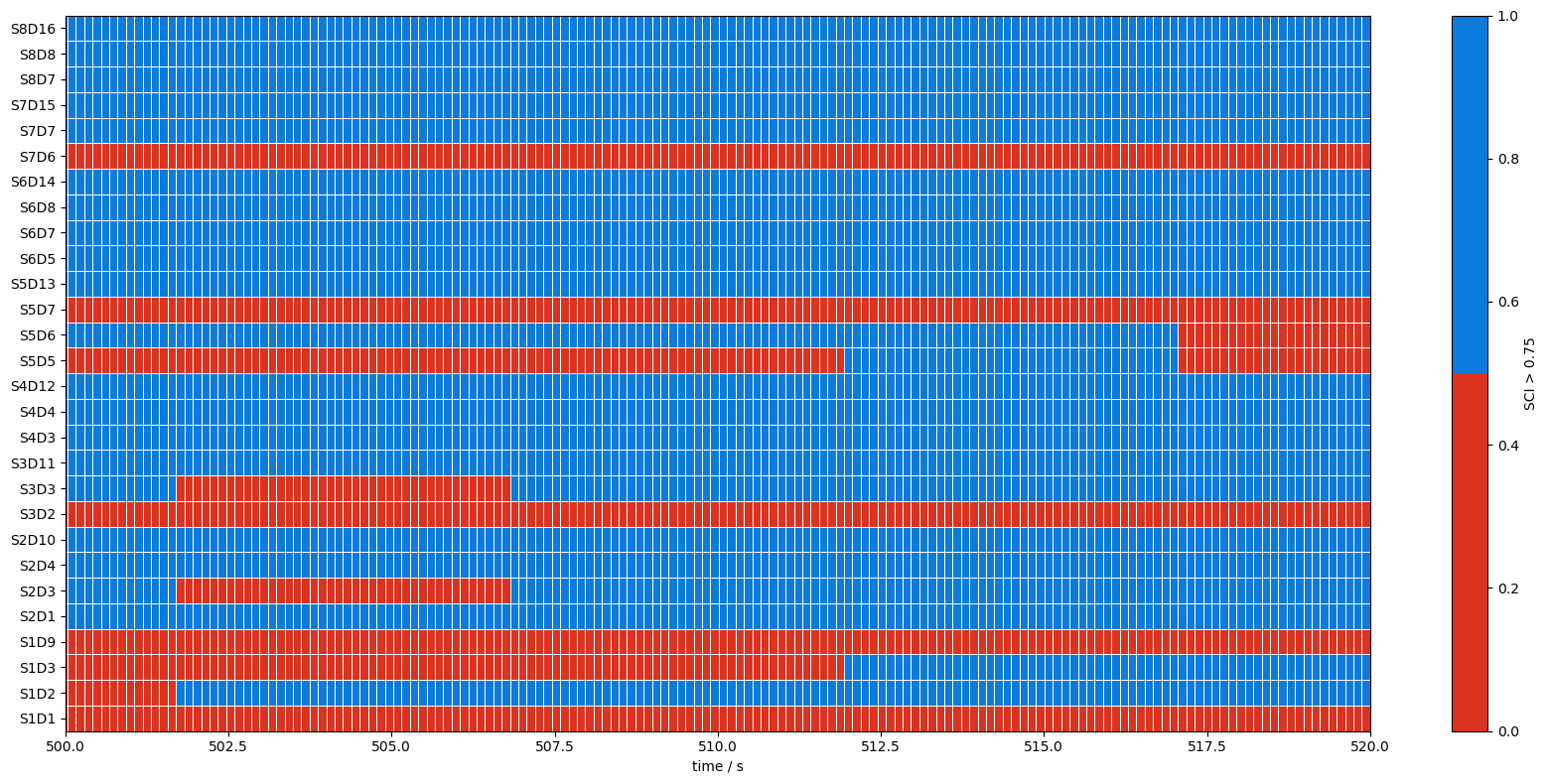
How to quantify signal quality (e.g. SCI, PSP, SNR, GVTD), build and combine quality masks, detect and correct motion artefacts, and assemble a complete preprocessing pipeline for a raw fNIRS dataset.
Content videos

4.1.C1 · Signal Quality: Concepts and Sources of Noise
4.2.C1 · Quality Metrics: Overview of Frequently Used Methods
4.3.C1 · Sources of Artifacts in fNIRS: Motion and Physiology
4.4.C1 · Practical Preprocessing: End-to-end Example of a Raw Dataset
Tutorial videos
Tutorial videos for this topic will show here as soon as they are recorded.
Example notebooks

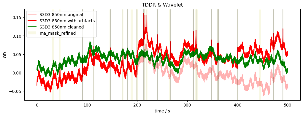
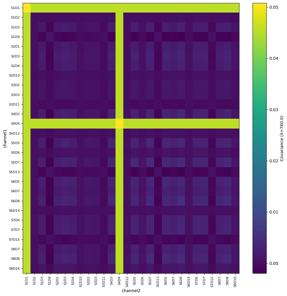

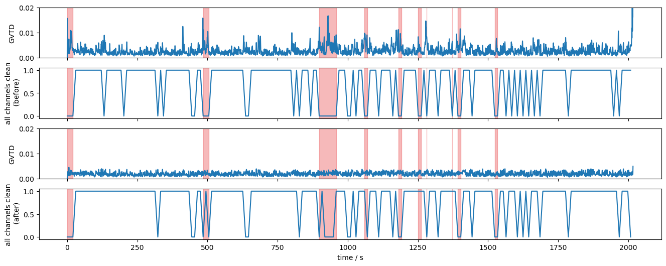
Related documentation: Signal processing · Physiology
5. General Linear Model (GLM)
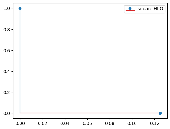
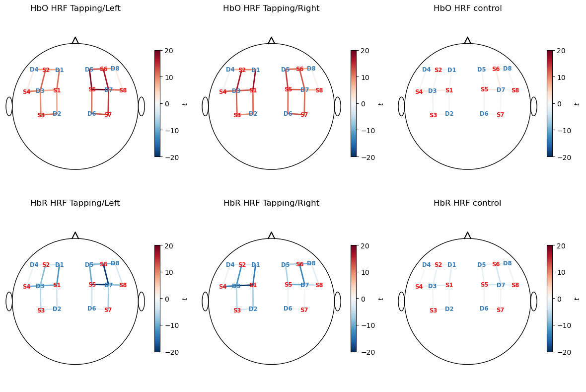
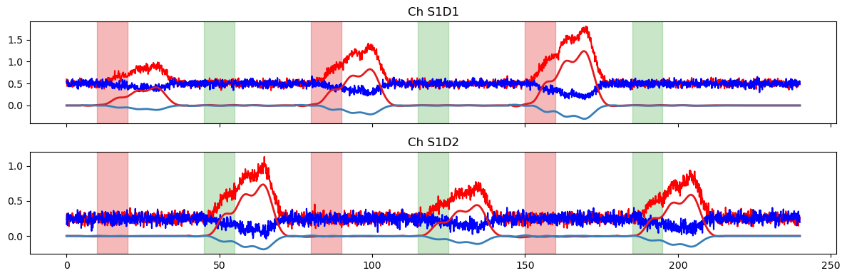
Modelling the haemodynamic response with the general linear model: design matrices with HRF basis functions, drift and short-channel regressors, the available solvers and noise models, and statistical inference on the estimated β values.
Content videos
5.1.C1 · GLM fundamentals: Short Channels, Physiology Regression and Introduction to the General Linear Model

5.2.C1 · GLM architecture in Cedalion
5.3.C1 · GLM Statistics: Statsmodels in Cedalion
Tutorial videos
Tutorial videos for this topic will show here as soon as they are recorded.
Example notebooks
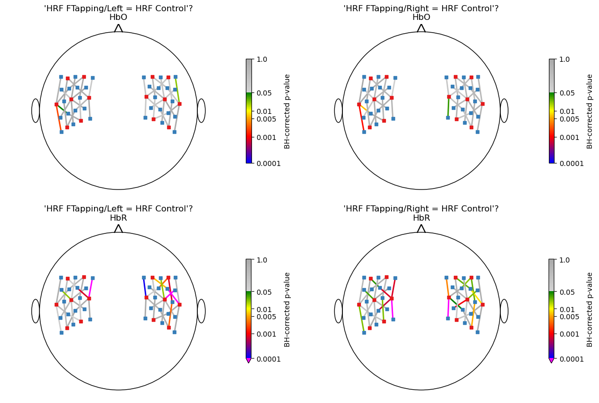
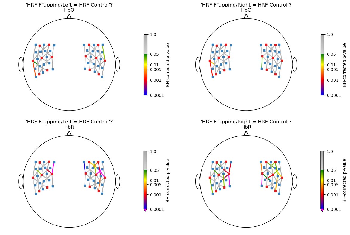
Related documentation: Modeling and machine learning
6. Head Models & Forward Modeling
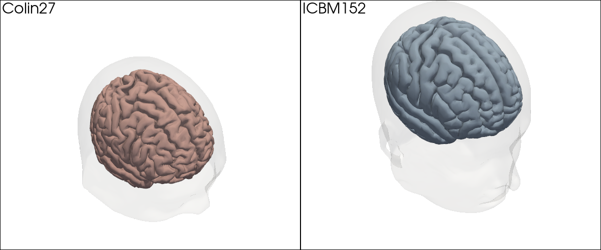
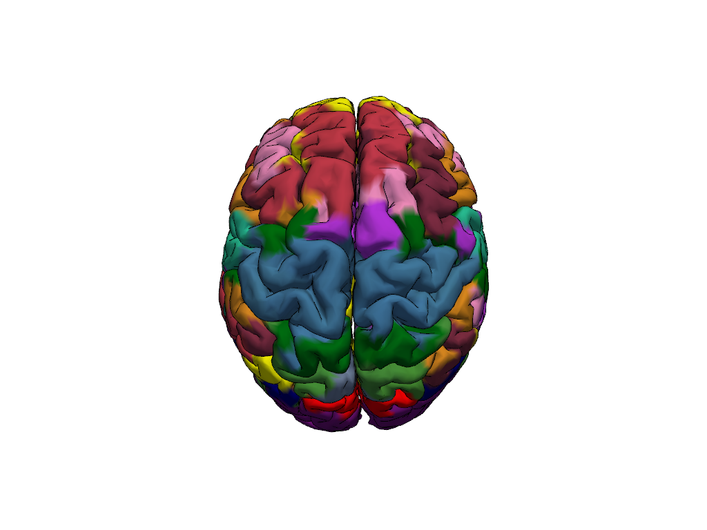
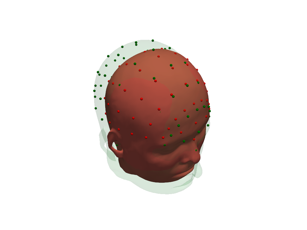
Head models describe the anatomy that light travels through. This section covers atlas-based and individual head models, coordinate systems, anatomical parcellations, and forward modelling with Monte Carlo (MCX) and finite-element (NIRFASTer) photon simulations.
Content videos
6.1.C1 · Head models in Neuroimaging: Overview
6.2.C1 · Overview of standard head-model coordinate systems
6.3.C1 · Forward modeling with photon simulations

6.4.C1 · Anatomical Atlases and Parcellation Schemes
Tutorial videos
Tutorial videos for this topic will show here as soon as they are recorded.
Example notebooks
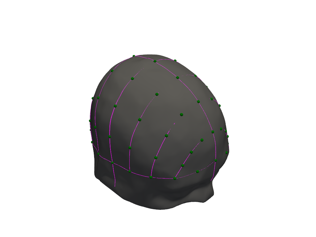
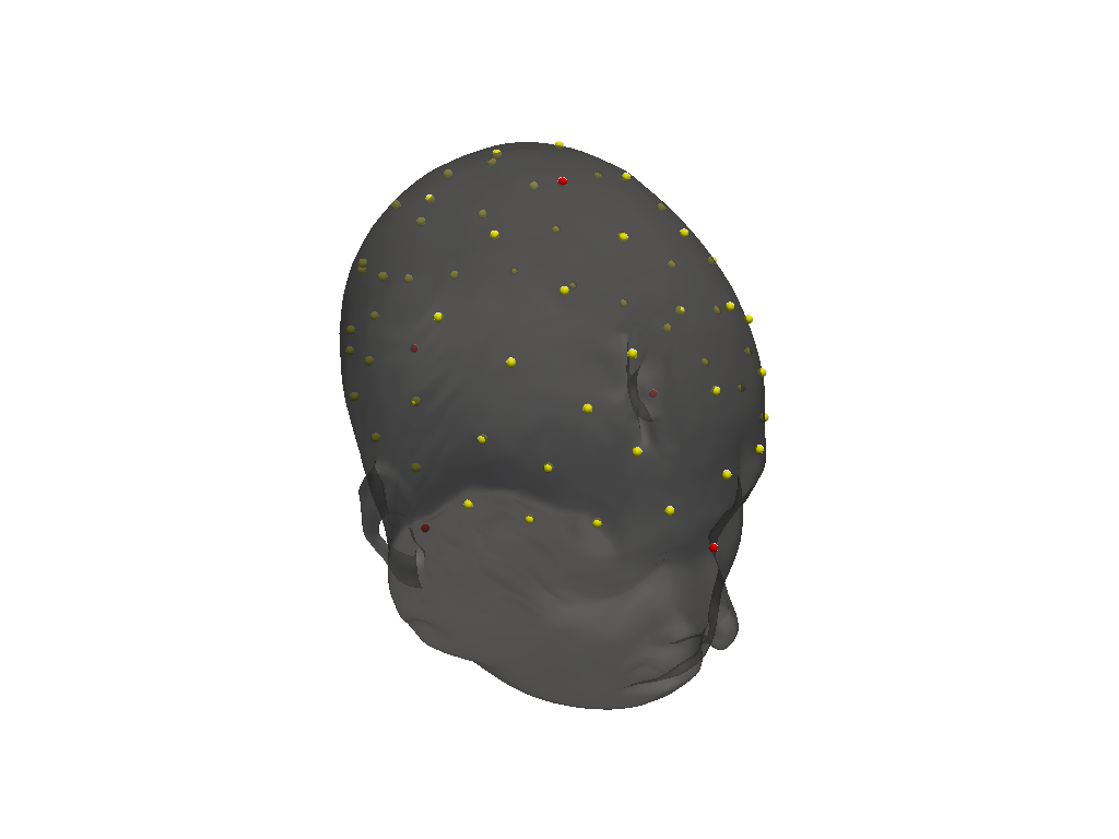


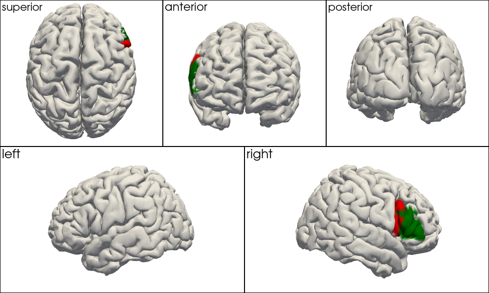
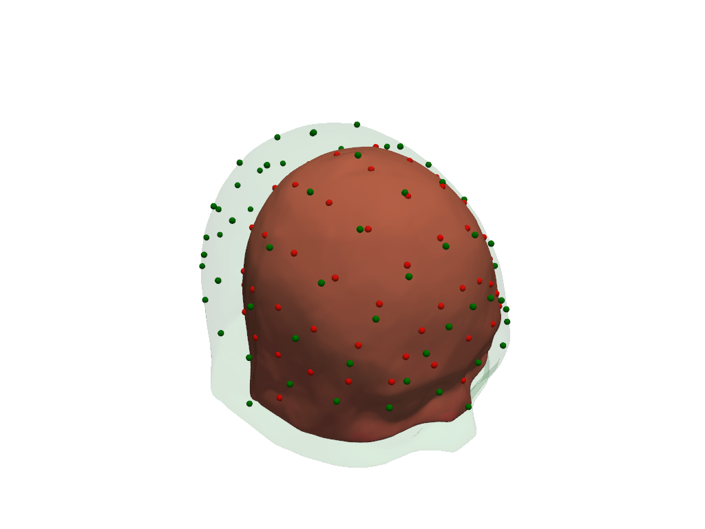
Related documentation: Diffuse optical tomography
7. Photogrammetric Optode Co-Registration & Probe Design
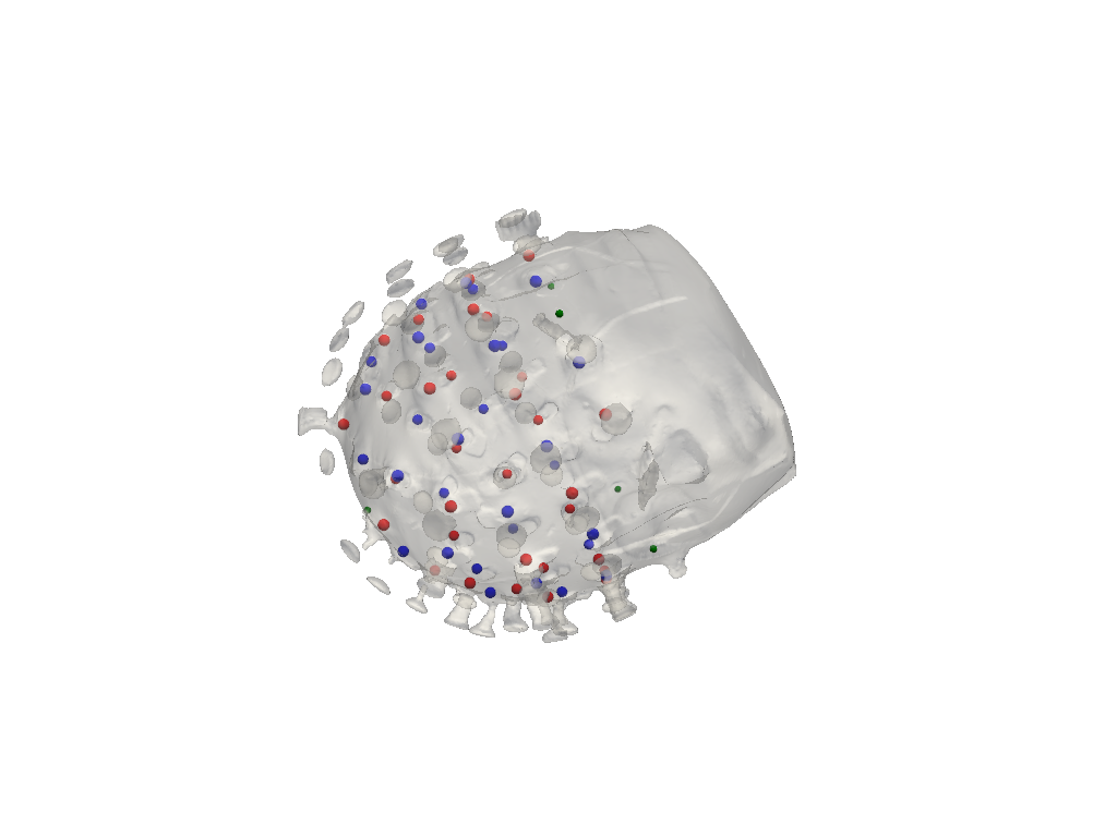
Photogrammetry measures where the optodes actually sit on a participant’s head. This section covers optode detection in 3D scans, manual quality control, and labelling the detected optodes by registering them to the probe layout. Tools for probe design are planned.
Content videos
7.1.C1 · Photogrammetry & co-registration: Motivation
7.2.C1 · Photogrammetric Optode Co-Registration in Cedalion

7.3.C1 · Probe Design in Cedalion
Tutorial videos
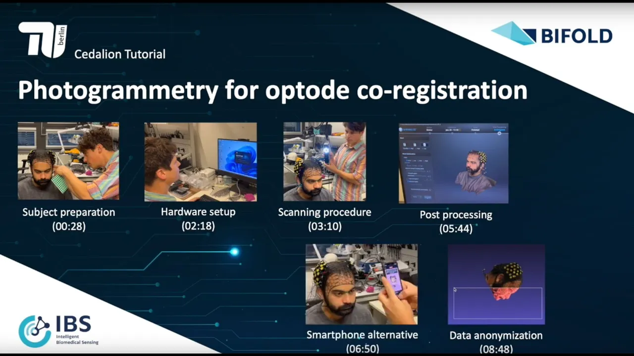
7.1.T1 · Acquiring and inspecting raw photogrammetry meshes
fNIRS/EEG photogrammetry tutorial with the Cedalion toolbox
More tutorial videos for this topic will show here as soon as they are recorded.
Example notebooks
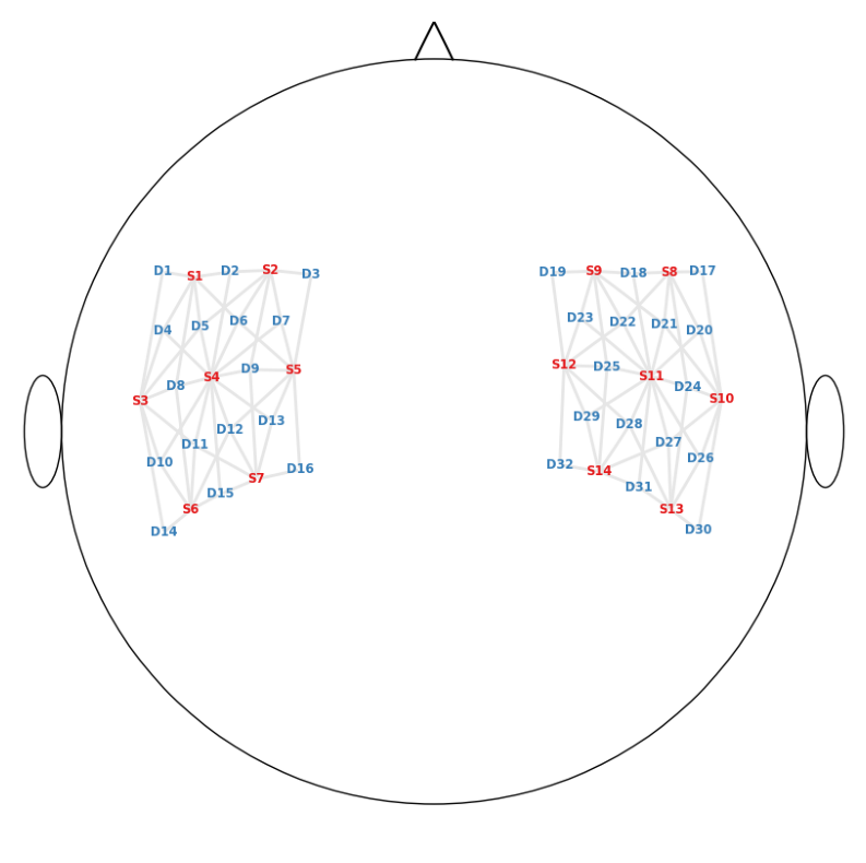
8. DOT Image Reconstruction
Diffuse optical tomography reconstructs images of cortical haemodynamic activity from channel-space measurements by inverting the sensitivity matrix. This section covers the inverse problem, regularisation choices, and aggregating images into brain parcels.
Content videos
8.1.C1 · Intro to DOT Image Reconstruction & Inverse Problem
8.2.C1 · Overview: Image Reconstruction workflow in Cedalion
Tutorial videos
Tutorial videos for this topic will show here as soon as they are recorded.
Example notebooks
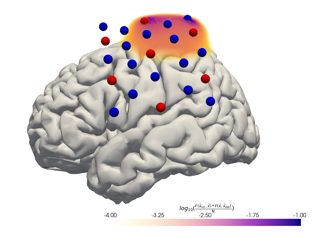
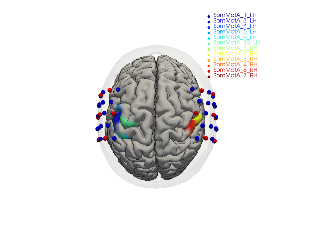
Related documentation: Diffuse optical tomography
9. Visualization & Interpretation
Cedalion’s plotting building blocks for time series, probe layouts, scalp and brain surfaces and reconstructed images, together with interactive tools for inspecting data.
Content videos
9.1.C1 · fNIRS/DOT visualization blocks in Cedalion
Tutorial videos
Tutorial videos for this topic will show here as soon as they are recorded.
Example notebooks
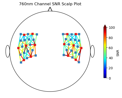
Related documentation: Plotting and visualization
10. Multimodal & Data-Driven Analysis
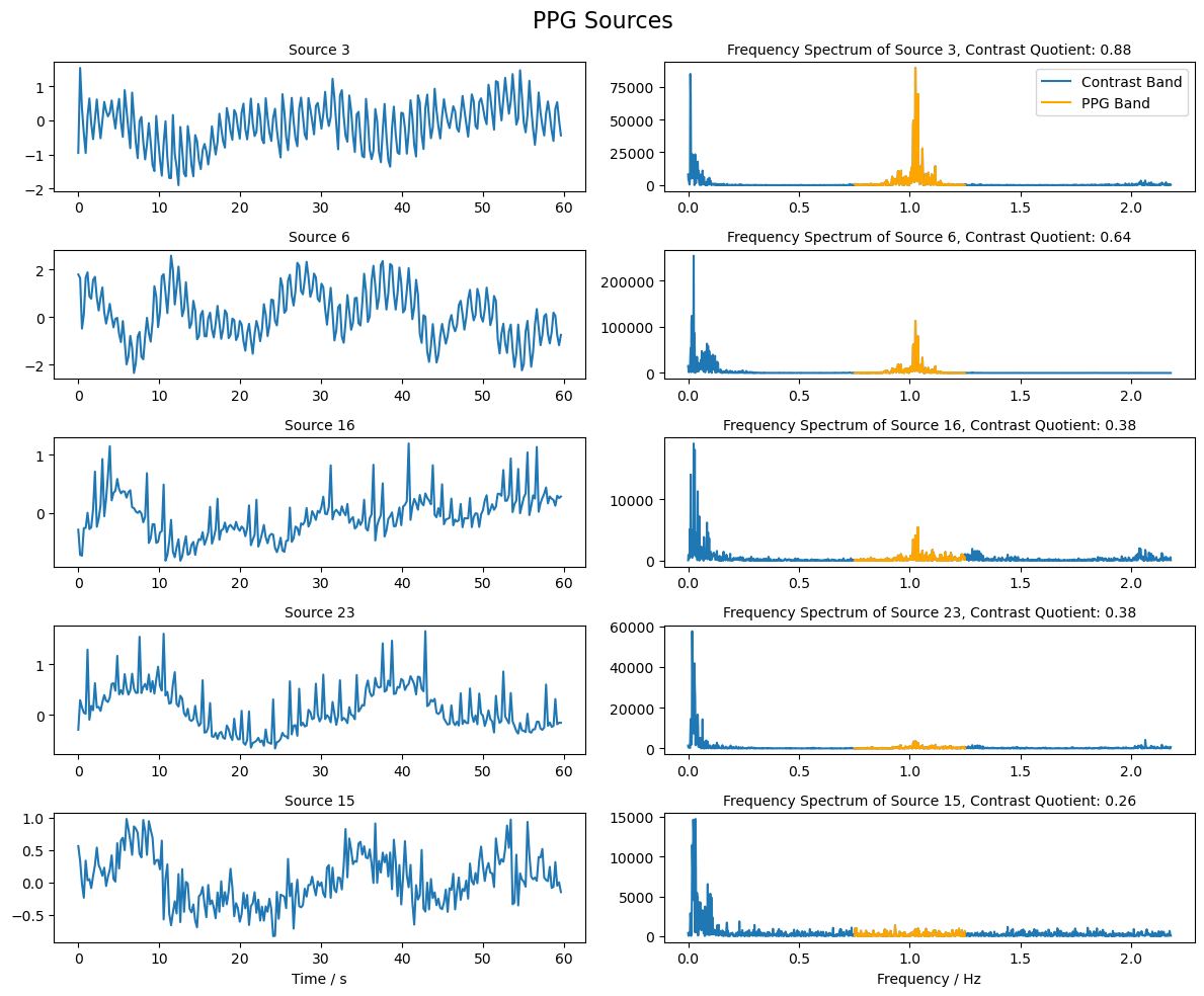
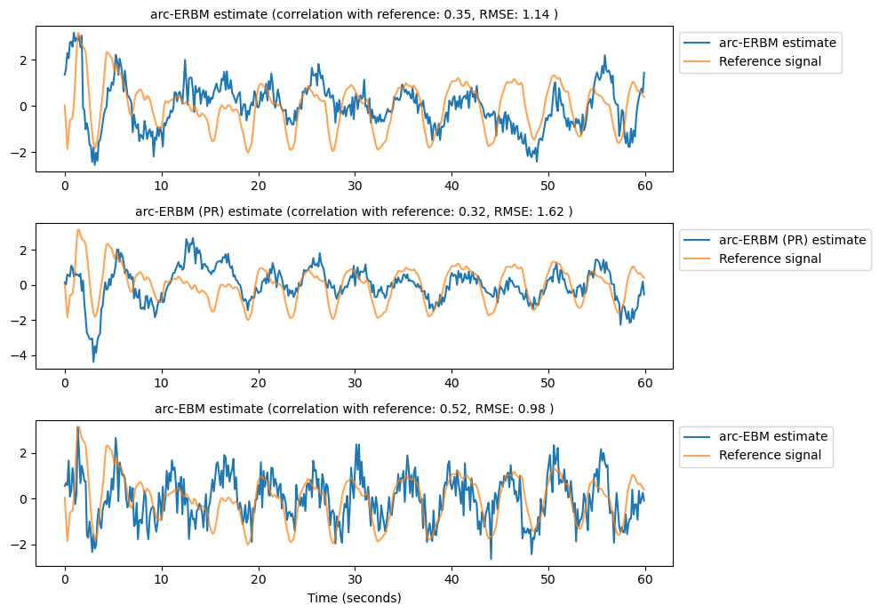
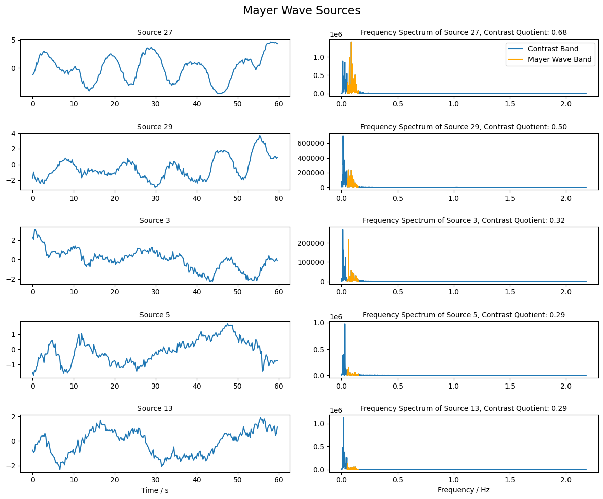
Data-driven methods that do not require a stimulus model: unimodal and multimodal source decomposition (ICA, the CCA family, mSPoC) and single-trial classification with scikit-learn.
Content videos
10.1.C1 · Multimodal fusion: variance vs decoding
10.2.C1 · Source Decomposition Methods Overview: CCA, ICA, SPoC family
10.3.C1 · ML fNIRS/DOT Classification Workflows
Tutorial videos
Tutorial videos for this topic will show here as soon as they are recorded.
Example notebooks

Related documentation: Modeling and machine learning
11. Simulation & Data Augmentation
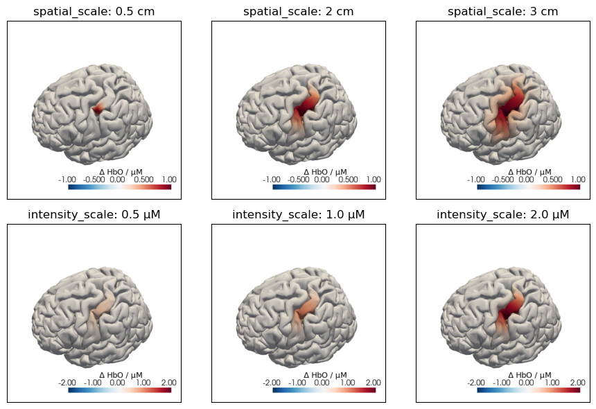
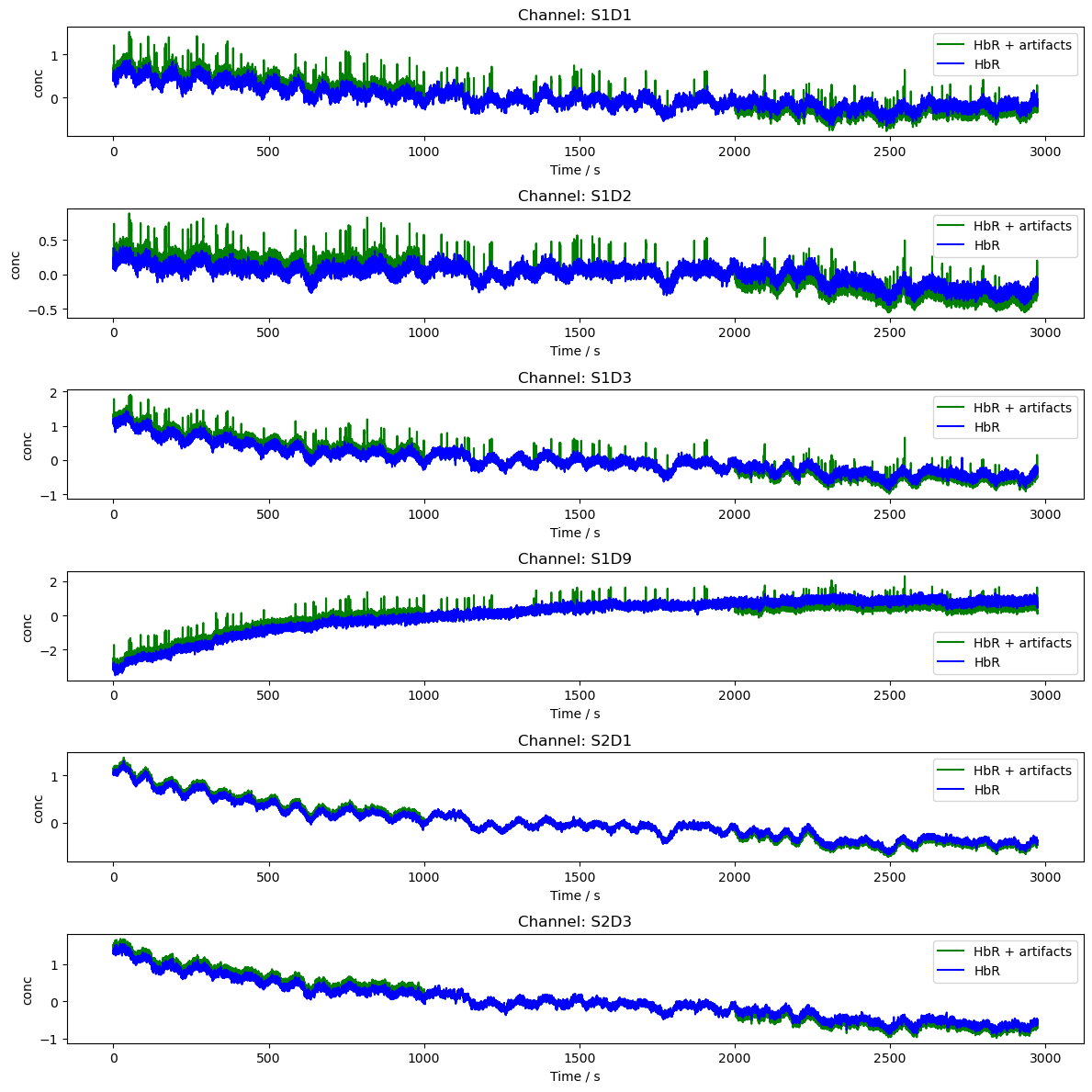
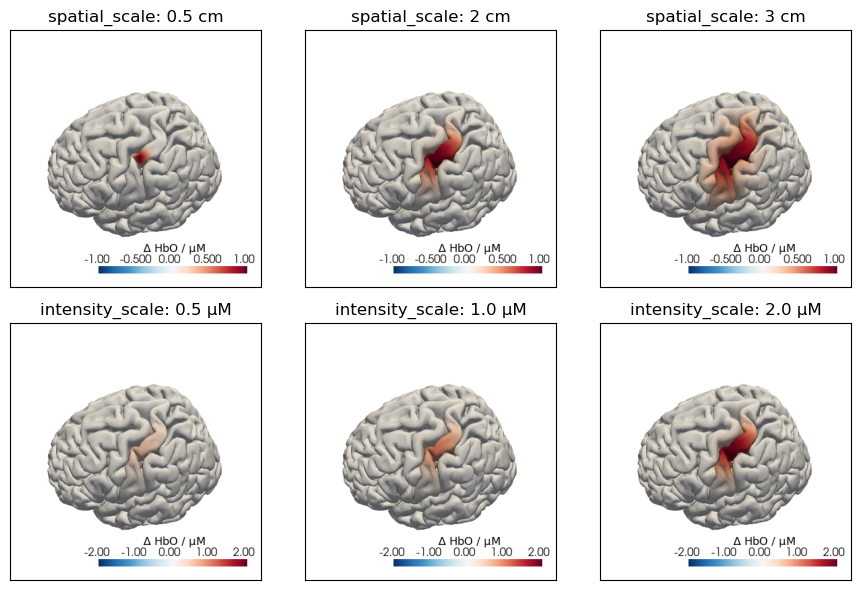
Synthetic haemodynamic responses, motion artefacts and paired fNIRS-EEG data with known ground truth, for benchmarking algorithms and augmenting training data for machine learning.
Content videos
11.1.C1 · Synthetic data for Benchmarking and Augmentation: Rationale

11.2.C1 · Synthetic data generation and augmentation in Cedalion
Tutorial videos
Tutorial videos for this topic will show here as soon as they are recorded.
Example notebooks
Related documentation: Synthetic data
12. Pipelines, Scaling & Reproducibility
Moving from interactive notebooks to scripted, reproducible pipelines that process many datasets and can be shared alongside a publication.
Content videos

12.1.C1 · Pipeline abstraction: From Notebooks to Pipelines
12.2.C1 · Snakemake integration in Cedalion: Concepts and Introduction
12.3.C1 · Reproducible and shareable Analyses
Tutorial videos
Tutorial videos for this topic will show here as soon as they are recorded.
Example notebooks
No example notebook covers this topic yet.
Related documentation: Environments · Changelog