Head Models in Cedalion: Getting Started

This notebook gives a practical introduction to head models in Cedalion. It is intended for users who are new to DOT/fNIRS head modeling and want to understand what a head model contains, how to load it, and how to inspect and visualize its components.

What you will learn:

Why head models are needed in fNIRS and DOT analysis
The two standard population atlases bundled with Cedalion: Colin27 and ICBM152
How to load a head model and what it contains
The link between the brain surface and FreeSurfer’s cortical reconstruction
How to visualize surfaces, landmarks, parcellations, and the inflated cortex
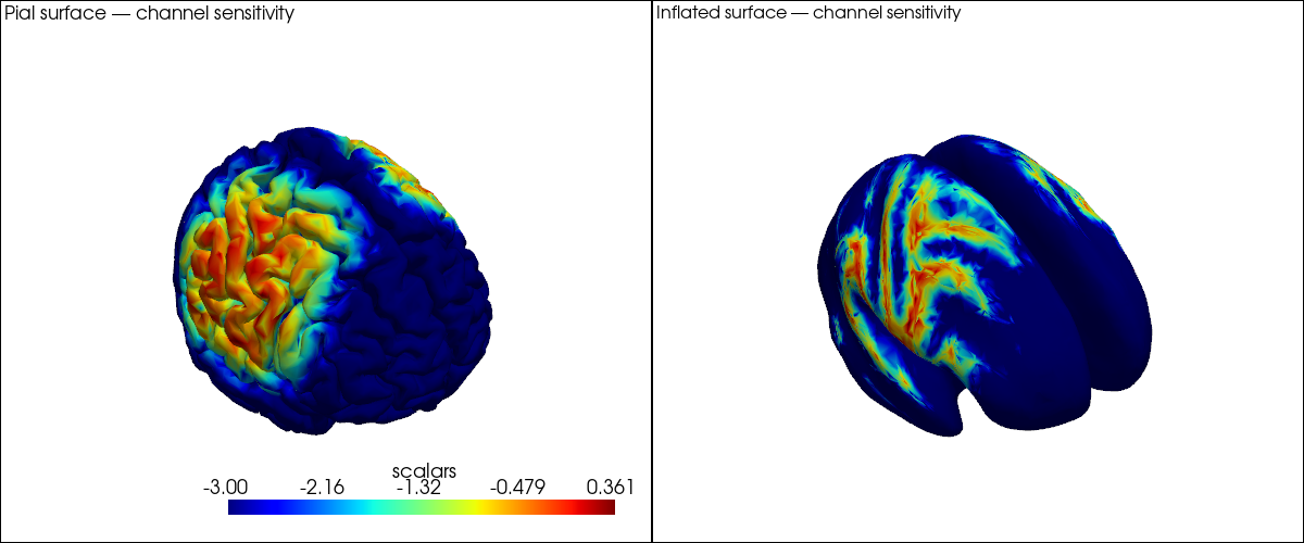
A first glimpse at channel sensitivity on the brain surface

For more detail, see:

40_image_reconstruction.ipynb — the full DOT image reconstruction pipeline
43b_individualized_head_models.ipynb — building a custom head model from individual MRI
44_head_models_crs_scaling.ipynb — coordinate systems, head scaling, optode registration
45_parcel_sensitivity.ipynb — parcel-level sensitivity analysis

[1]:

# This cell sets up the environment when executed in Google Colab.
try:
    import google.colab
    !curl -s https://raw.githubusercontent.com/ibs-lab/cedalion/dev/scripts/colab_setup.py -o colab_setup.py
    %run colab_setup.py
except ImportError:
    pass

[2]:

import numpy as np
import xarray as xr
import pyvista as pv

import cedalion
import cedalion.data
import cedalion.dot
import cedalion.dataclasses as cdc
import cedalion.vis.blocks as vbx

# Use 'server' for interactive 3-D rotation in a local Jupyter session.
# Use 'static' for rendered documentation or environments without a display.
pv.set_jupyter_backend('static')

xr.set_options(display_expand_data=False);

1. Why Do We Need a Head Model?

In fNIRS and DOT, light is emitted from a source optode on the scalp, travels through several tissue layers (skin, skull, cerebrospinal fluid, cortex), and is detected at a detector optode nearby. The measured signal is therefore a spatially blurred mixture of absorption changes from all tissues the light passed through.

A head model provides the anatomical context needed to:

Register optode positions to the head surface.
Simulate light propagation through tissue (forward model).
Map channel-space signals back to brain-surface locations (image reconstruction).

In Cedalion, a head model is represented by the TwoSurfaceHeadModel class. It bundles:

Component	Description
`brain`	Triangulated cortical surface mesh
`scalp`	Triangulated scalp surface mesh
`segmentation_masks`	Voxel-wise tissue labels (scalp, skull, CSF, GM, WM)
`landmarks`	Fiducial points (Nz, Iz, Cz, LPA, RPA) for registration
`t_ijk2ras`	Affine transform from voxel to physical (RAS) space

The brain surface vertices carry additional coordinates that link them back to FreeSurfer’s cortical parcellation — more on that in Section 4.

2. The Two Standard Atlases: Colin27 and ICBM152

Cedalion ships with two standard population atlases, both fully processed and ready to use without any MRI data of your own.

Colin27 is built from 27 MRI scans of a single individual averaged together. The high number of averages yields exceptional anatomical detail and signal-to-noise ratio, making it a popular reference. Because it is a single subject, however, it may not be representative of a broader population.

ICBM152 is an average over 152 healthy adult brains from the International Consortium for Brain Mapping. Its anatomy is somewhat blurred by the averaging but it is more representative for group studies.

Both atlases were processed with FreeSurfer for cortical surface reconstruction and labelled with the Schaefer2018 parcellation scheme. They share the same data structure and API.

[3]:

# Load both standard atlases. The files are downloaded automatically on first use
# and cached locally. Subsequent calls load from the cache.
head_colin = cedalion.dot.get_standard_headmodel("colin27")
head_icbm  = cedalion.dot.get_standard_headmodel("icbm152")

[4]:

# Side-by-side comparison: scalp (transparent) + brain surface for each atlas.
plt = pv.Plotter(shape=(1, 2), window_size=(1200, 500))

plt.subplot(0, 0)
plt.add_text("Colin27", position="upper_left", font_size=12)
vbx.plot_surface(plt, head_colin.brain, color="#d3a6a1")
vbx.plot_surface(plt, head_colin.scalp, color="w", opacity=0.1)

plt.subplot(0, 1)
plt.add_text("ICBM152", position="upper_left", font_size=12)
vbx.plot_surface(plt, head_icbm.brain, color="#a1b8d3")
vbx.plot_surface(plt, head_icbm.scalp, color="w", opacity=0.1)

plt.link_views()
plt.show()

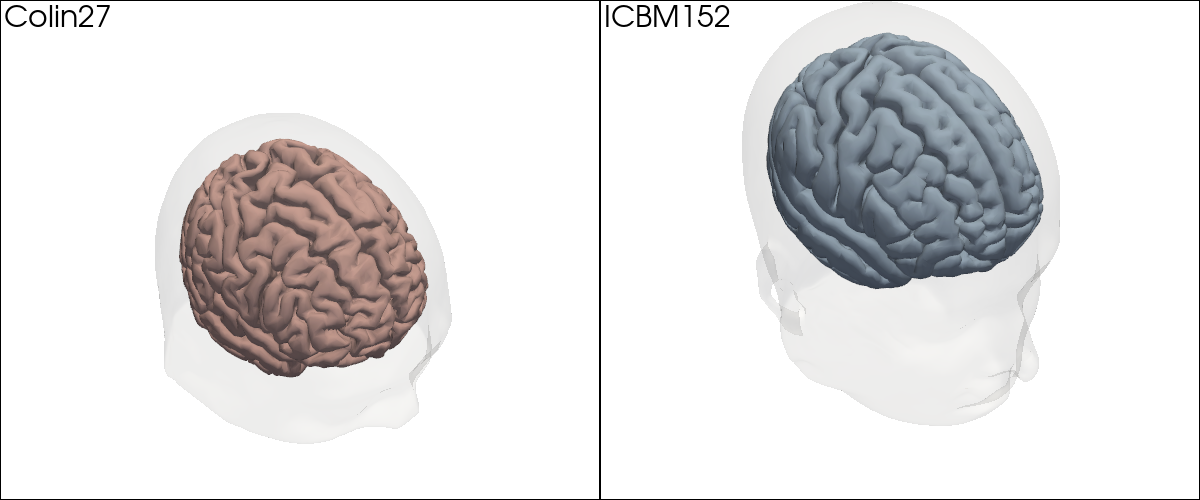
../../_images/examples_head_models_43a_head_models_overview_6_0.png

The two atlases look similar overall; the finer gyral detail in Colin27 is visible when you zoom in. For the remainder of this notebook we will work with Colin27.

3. What Is Inside a Head Model?

Let us load the Colin27 head model and inspect each of its components in turn. The model is loaded in voxel space (crs='ijk'), where each voxel has unit edge length and coordinates are dimensionless. We will convert to physical space in Section 6.

[5]:

head_ijk = cedalion.dot.get_standard_headmodel("colin27")
head_ijk

[5]:

TwoSurfaceHeadModel(
  crs: ijk
  tissue_types: csf, gm, scalp, skull, wm
  brain faces: 49992 vertices: 25000 units: dimensionless
  scalp faces: 20096 vertices: 10050 units: dimensionless
  landmarks: 73
)

[6]:

# The brain surface is a TrimeshSurface: a triangulated mesh with vertices and faces.
# Each vertex carries additional coordinates — we will explore these in Section 4.
head_ijk.brain

[6]:

TrimeshSurface(faces: 49992 vertices: 25000 crs: ijk units: dimensionless vertex_coords: ['fsaverage_vertex', 'parcel', 'mni152_r', 'mni152_a', 'mni152_s'])

[7]:

# The scalp surface encloses the entire head.
head_ijk.scalp

[7]:

TrimeshSurface(faces: 20096 vertices: 10050 crs: ijk units: dimensionless vertex_coords: [])

[8]:

# Segmentation masks: a 3-D voxel array labelling each voxel as one of five tissue types.
head_ijk.segmentation_masks

[8]:

<xarray.DataArray (segmentation_type: 5, i: 181, j: 217, k: 181)> Size: 36MB
0 0 0 0 0 0 0 0 0 0 0 0 0 0 0 0 0 0 0 ... 0 0 0 0 0 0 0 0 0 0 0 0 0 0 0 0 0 0 0
Coordinates:
  * segmentation_type  (segmentation_type) <U5 100B 'csf' 'gm' ... 'skull' 'wm'
Dimensions without coordinates: i, j, k

[9]:

# Landmarks: five fiducial points used for optode registration and head scaling.
head_ijk.landmarks

[9]:

<xarray.DataArray (label: 73, ijk: 3)> Size: 2kB
[] 90.0 7.435 48.92 3.924 106.0 24.01 ... 127.4 25.63 109.0 139.8 26.66 93.47
Coordinates:
  * label    (label) <U3 876B 'Iz' 'LPA' 'RPA' 'Nz' ... 'PO1' 'PO2' 'PO4' 'PO6'
    type     (label) object 584B PointType.LANDMARK ... PointType.LANDMARK
Dimensions without coordinates: ijk

[10]:

# The affine transformation that converts voxel coordinates to physical (RAS) space.
head_ijk.t_ijk2ras

[10]:

<xarray.DataArray (mni: 4, ijk: 4)> Size: 128B
[mm] 1.0 0.0 0.0 -90.0 0.0 1.0 0.0 -126.0 0.0 0.0 1.0 -72.0 0.0 0.0 0.0 1.0
Dimensions without coordinates: mni, ijk

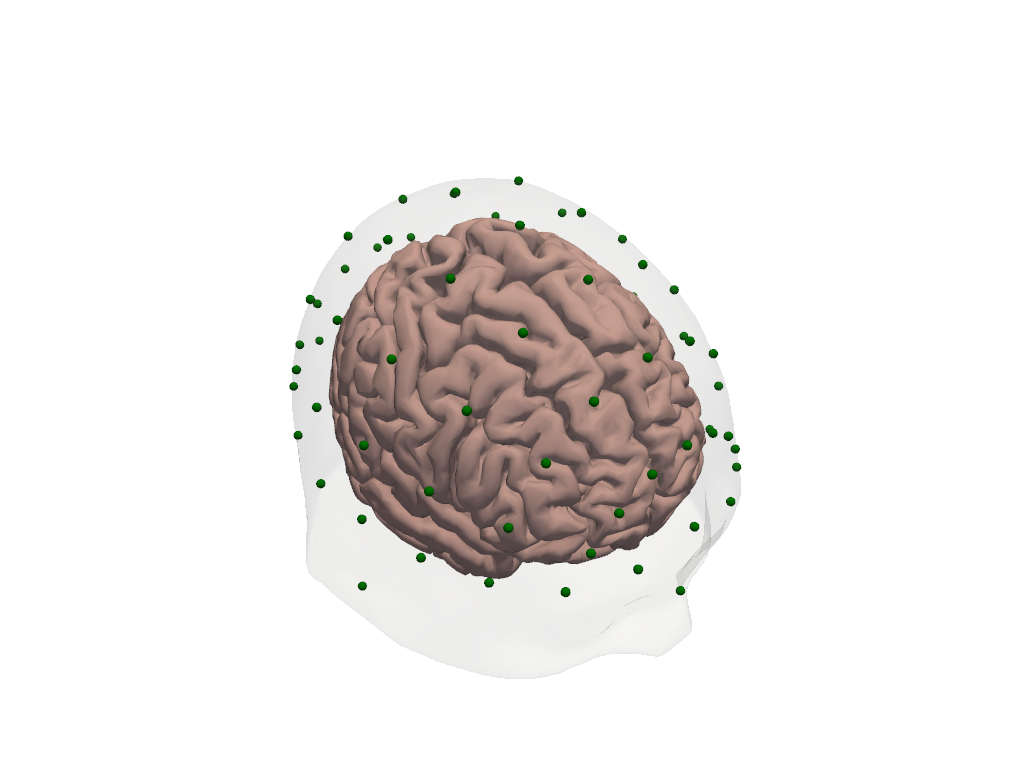
[11]:

# Visualize the head model: transparent scalp, brain surface, and labelled landmarks.
plt = pv.Plotter()
vbx.plot_surface(plt, head_ijk.brain, color="#d3a6a1")
vbx.plot_surface(plt, head_ijk.scalp, color="w", opacity=0.12)
vbx.plot_labeled_points(plt, head_ijk.landmarks, show_labels=True)
plt.show()

../../_images/examples_head_models_43a_head_models_overview_15_0.png

4. Under the Hood: HeadModelFiles and the FreeSurfer Connection

The atlas data is stored on disk as a collection of files. get_colin27_headmodel_files() returns a HeadModelFiles object that lists every file in the bundle and provides convenience loaders for the ones that are used most often.

[12]:

hmfiles = cedalion.data.get_colin27_headmodel_files()
hmfiles

[12]:

HeadModelFiles(basedir=PosixPath('/home/runner/.cache/cedalion/dev/hm_colin27.zip.unzip/hm_colin27'), mask_files={'csf': 'mask_csf.nii', 'gm': 'mask_gray.nii', 'scalp': 'mask_skin.nii', 'skull': 'mask_bone.nii', 'wm': 'mask_white.nii'}, landmarks_ras_file='landmarks.mrk.json', brain_vertex_coordinates='brain_vertex_coordinates.csv', scalp_surface_obj='mask_scalp.obj', brain_surface_obj='mask_brain.obj', freesurfer_surface_obj='cortex_pial_high.obj', inflated_surface_obj='cortex_pial_inflated.obj', parcel_colors='parcel_colors.json', voxel_to_vertex_mapping='voxel_to_vertex_brain.mtx.gz')

The key file here is brain_vertex_coordinates. It is a table with one row per brain surface vertex and four columns that link the vertex to its anatomical context:

[13]:

vertex_coords = hmfiles.load_brain_vertex_coordinates()
vertex_coords

[13]:

	vertex	fsaverage_vertex	parcel	mni152_r	mni152_a	mni152_s
0	0	42	VisCent_ExStr_8_LH	-6.792	-104.805	-1.408
1	1	61	VisCent_Striate_2_LH	-5.846	-104.306	-3.845
2	2	75	VisCent_ExStr_8_LH	-10.867	-104.149	-6.014
3	3	89	VisCent_ExStr_8_LH	-13.822	-103.441	7.414
4	4	96	VisCent_Striate_2_LH	-5.653	-103.617	5.033
...	...	...	...	...	...	...
24995	24995	332996	VisPeri_ExStrInf_1_RH	18.443	-46.567	-10.676
24996	24996	333005	VisCent_ExStr_9_RH	16.206	-101.148	-6.879
24997	24997	333018	ContA_PFCl_5_RH	37.180	28.708	27.921
24998	24998	333020	Background+FreeSurfer_Defined_Medial_Wall	6.633	-19.161	15.987
24999	24999	333066	VisCent_ExStr_7_RH	37.946	-89.492	-10.045

25000 rows × 6 columns

Each column carries specific meaning:

Column	Meaning
`vertex`	Index in the (downsampled) Cedalion brain mesh
`fsaverage_vertex`	Corresponding vertex index in FreeSurfer’s `fsaverage` template (~330 000 vertices)
`parcel`	Schaefer2018 parcel label assigned to this vertex
`mni152_r/a/s`	MNI152 RAS coordinates of the vertex in mm

The fsaverage_vertex index is the key that links this downsampled surface back to the full-resolution FreeSurfer reconstruction and enables comparison across subjects or atlases: any vertex in Colin27 can be mapped to the same anatomical location in ICBM152 via the shared fsaverage space.

These columns are not just metadata stored in a file — they are attached as coordinates directly on the brain.vertices xarray DataArray, so they are always available when working with the brain surface:

[14]:

# All vertex coordinates are accessible as xarray coords on the brain surface.
head_ijk.brain.vertices

[14]:

<xarray.DataArray (label: 25000, ijk: 3)> Size: 600kB
[] 82.52 19.84 68.31 83.52 20.32 65.89 ... 96.28 105.3 86.73 127.6 34.46 60.38
Coordinates:
  * label             (label) int64 200kB 0 1 2 3 4 ... 24996 24997 24998 24999
  * fsaverage_vertex  (label) int64 200kB 42 61 75 89 ... 333018 333020 333066
  * parcel            (label) object 200kB 'VisCent_ExStr_8_LH' ... 'VisCent_...
  * mni152_r          (label) float64 200kB -6.792 -5.846 -10.87 ... 6.633 37.95
  * mni152_a          (label) float64 200kB -104.8 -104.3 ... -19.16 -89.49
  * mni152_s          (label) float64 200kB -1.408 -3.845 ... 15.99 -10.04
Dimensions without coordinates: ijk

5. Brain Surface Parcellations and the Inflated Cortex

The Schaefer2018 atlas divides the cortex into functional regions (parcels) derived from resting-state fMRI connectivity. With ~400–600 parcels (depending on resolution), it provides a rich labelling of the cortex that is useful for ROI-level analysis and for reporting results in a standardised anatomical vocabulary.

Since each brain surface vertex already carries its parcel label as a coordinate, we can colour the mesh directly by parcel — no additional lookup is needed.

[15]:

# Load the RGB colour map for the Schaefer parcellation.
parcel_colors = hmfiles.load_parcel_colors()

# Each entry is a parcel name -> [R, G, B] list (0-255 range).
# Show a small sample.
dict(list(parcel_colors.items())[:5])

[15]:

{'VisCent_Striate_1_LH': [120, 18, 135],
 'VisCent_Striate_2_LH': [120, 18, 136],
 'VisCent_Striate_3_LH': [120, 18, 137],
 'VisCent_ExStr_1_LH': [120, 18, 128],
 'VisCent_ExStr_2_LH': [120, 18, 129]}

[16]:

# Build a per-vertex colour list from the parcel labels on the brain surface.
vertex_colors = [
    parcel_colors.get(pc, [180, 180, 180])
    for pc in head_ijk.brain.vertices.parcel.values
]

plt = pv.Plotter()
vbx.plot_surface(plt, head_ijk.brain, color=vertex_colors)
plt.show()

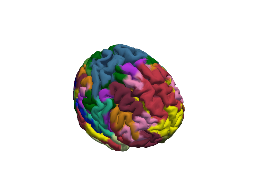
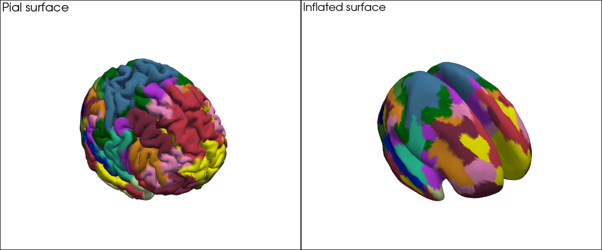
../../_images/examples_head_models_43a_head_models_overview_24_0.png

With ~400 parcels the individual region boundaries are hard to see on the folded surface. This is where the inflated cortex helps: the surface is computationally inflated to remove sulci and gyri while preserving the vertex layout. Every vertex keeps exactly the same index and coordinates — only the 3-D positions change — so the same colour vector applies directly to the inflated mesh.

[17]:

infl_mesh = cedalion.dot.get_inflated_cortex_surface("colin27")
infl_mesh

[17]:

TrimeshSurface(faces: 49992 vertices: 25000 crs: inflated units: dimensionless vertex_coords: [])

[18]:

# Parcellations on the pial (folded) surface vs. the inflated surface, side by side.
plt = pv.Plotter(shape=(1, 2), window_size=(1200, 500))

plt.subplot(0, 0)
plt.add_text("Pial surface", position="upper_left", font_size=11)
vbx.plot_surface(plt, head_ijk.brain, color=vertex_colors)

plt.subplot(0, 1)
plt.add_text("Inflated surface", position="upper_left", font_size=11)
vbx.plot_surface(plt, infl_mesh, color=vertex_colors)

plt.show()

../../_images/examples_head_models_43a_head_models_overview_27_0.png

Highlighting Specific Parcels

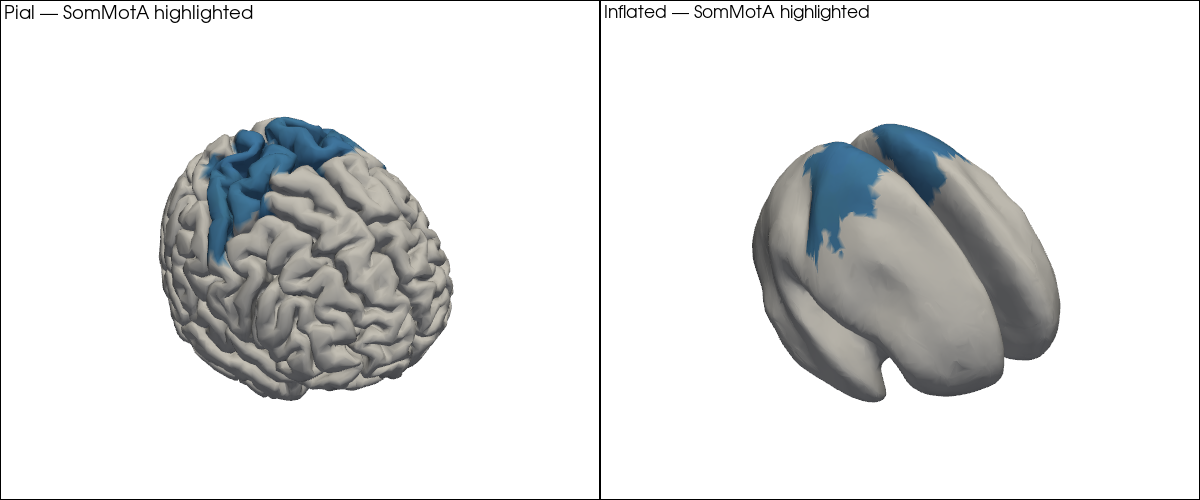
In practice, you will often want to highlight a specific set of parcels — for example the bilateral primary somatomotor cortex (SomMotA) when analysing a motor task. The code pattern is the same: build the per-vertex colour list, but set unselected vertices to grey.

[19]:

# Select bilateral somatomotor parcels as an example.
selected_parcels = [p for p in parcel_colors if "SomMotA" in p]
print(f"{len(selected_parcels)} parcels selected: {selected_parcels[:6]} ...")

56 parcels selected: ['SomMotA_1_LH', 'SomMotA_2_LH', 'SomMotA_3_LH', 'SomMotA_4_LH', 'SomMotA_5_LH', 'SomMotA_6_LH'] ...

[20]:

selected_colors = {p: c for p, c in parcel_colors.items() if p in selected_parcels}

highlight_colors = [
    selected_colors.get(pc, [210, 210, 210])
    for pc in head_ijk.brain.vertices.parcel.values
]

plt = pv.Plotter(shape=(1, 2), window_size=(1200, 500))

plt.subplot(0, 0)
plt.add_text("Pial — SomMotA highlighted", position="upper_left", font_size=10)
vbx.plot_surface(plt, head_ijk.brain, color=highlight_colors)

plt.subplot(0, 1)
plt.add_text("Inflated — SomMotA highlighted", position="upper_left", font_size=10)
vbx.plot_surface(plt, infl_mesh, color=highlight_colors)

plt.show()

../../_images/examples_head_models_43a_head_models_overview_30_0.png

6. Coordinate Systems in 60 Seconds

The head model is loaded in voxel space (crs='ijk'): axis-aligned, dimensionless integer-like coordinates. This is the native space for the photon simulation code (MCX, NIRFASTERff. etc.).

For optode registration, visualisation alongside physical measurements, or comparison with MNI-space atlas coordinates, you need physical (RAS) space. The affine transformation t_ijk2ras converts between the two. Applying it to the head model transforms every component — surfaces, landmarks, and the transform itself — simultaneously.

[21]:

print(f"CRS before transform: '{head_ijk.crs}'")
print(f"Landmark units before: {head_ijk.landmarks.pint.units}")

head_ras = head_ijk.apply_transform(head_ijk.t_ijk2ras)

print(f"\nCRS after transform:  '{head_ras.crs}'")
print(f"Landmark units after:  {head_ras.landmarks.pint.units}")

CRS before transform: 'ijk'
Landmark units before: dimensionless

CRS after transform:  'mni'
Landmark units after:  millimeter

[22]:

# Landmarks in physical (mm) space.
head_ras.landmarks

[22]:

<xarray.DataArray (label: 73, mni: 3)> Size: 2kB
[mm] 0.0045 -118.6 -23.08 -86.08 -19.99 ... -100.4 37.02 49.81 -99.34 21.47
Coordinates:
  * label    (label) <U3 876B 'Iz' 'LPA' 'RPA' 'Nz' ... 'PO1' 'PO2' 'PO4' 'PO6'
    type     (label) object 584B PointType.LANDMARK ... PointType.LANDMARK
Dimensions without coordinates: mni

[23]:

# Visualize head in RAS space — axes are now in mm.
plt = pv.Plotter()
vbx.plot_surface(plt, head_ras.brain, color="#d3a6a1")
vbx.plot_surface(plt, head_ras.scalp, color="w", opacity=0.1)
vbx.plot_labeled_points(plt, head_ras.landmarks, show_labels=True)
plt.show()

../../_images/examples_head_models_43a_head_models_overview_34_0.png

For a full treatment of coordinate systems — including scaling the head model to a subject’s measured head size and snapping digitized optode positions to the scalp surface — see 44_head_models_crs_scaling.ipynb.

8. Where to Go Next

You have now seen the key building blocks of Cedalion head models. Here is a map to the rest of the head model notebook series:

Notebook	What it covers
44_head_models_crs_scaling.ipynb	Coordinate systems in depth; scaling the head model to a subject’s head size; registering and snapping digitized optode positions to the scalp
43b_individualized_head_models.ipynb	Building a custom head model from an individual T1 MRI using FreeSurfer, CAT12, and the Schaefer parcellation pipeline
40_image_reconstruction.ipynb	Full DOT pipeline: preprocessing, optode registration, Monte Carlo forward model, image reconstruction, and visualization
45_parcel_sensitivity.ipynb	Parcel-level sensitivity analysis: which brain regions does a given montage cover?
46_precompute_fluence.ipynb	Pre-computing and caching fluence files for large montages

References

[27]:

cedalion.bib.dump_to_notebook()

Methods used

[1]	Holmes1998	cedalion.data.get_colin27_headmodel_files	Colin J. Holmes, Rick Hoge, Louis Collins, Roger Woods, Arthur W. Toga, and Alan C. Evans. Enhancement of mr images using registration for signal averaging. Journal of Computer Assisted Tomography, 22(2):324–333, March 1998. doi:10.1097/00004728-199803000-00032.
[2]	Fischl2012	cedalion.data.get_colin27_headmodel_files, cedalion.data.get_icbm152_headmodel_files	Bruce Fischl. FreeSurfer. NeuroImage, 62(2):774–781, 2012. doi:10.1016/j.neuroimage.2012.01.021.
[3]	Schaefer2018	cedalion.data.get_colin27_headmodel_files, cedalion.data.get_icbm152_headmodel_files	Alexander Schaefer, Ru Kong, Evan M Gordon, Timothy O Laumann, Xi-Nian Zuo, Avram J Holmes, Simon B Eickhoff, and BT Thomas Yeo. Local-global parcellation of the human cerebral cortex from intrinsic functional connectivity mri. Cerebral cortex, 28(9):3095–3114, 2018. doi:10.1093/cercor/bhx179.
[4]	Fonov2011	cedalion.data.get_icbm152_headmodel_files	Vladimir Fonov, Alan C. Evans, Kelly Botteron, C. Robert Almli, Robert C. McKinstry, and D. Louis Collins. Unbiased average age-appropriate atlases for pediatric studies. NeuroImage, 54(1):313–327, January 2011. doi:10.1016/j.neuroimage.2010.07.033.
[5]	Fang2009	cedalion.data.get_precomputed_sensitivity	Qianqian Fang and David A Boas. Monte carlo simulation of photon migration in 3d turbid media accelerated by graphics processing units. Optics express, 17(22):20178–20190, 2009. doi:10.1364/OE.17.020178.
[6]	Yu2018	cedalion.data.get_precomputed_sensitivity	Leiming Yu, Fanny Nina-Paravecino, David Kaeli, and Qianqian Fang. Scalable and massively parallel monte carlo photon transport simulations for heterogeneous computing platforms. Journal of biomedical optics, 23(1):010504–010504, 2018. doi:10.1117/1.JBO.23.1.010504.
[7]	Yan2020	cedalion.data.get_precomputed_sensitivity	Shijie Yan and Qianqian Fang. Hybrid mesh and voxel based monte carlo algorithm for accurate and efficient photon transport modeling in complex bio-tissues. Biomedical Optics Express, 11(11):6262–6270, 2020. doi:10.1364/BOE.409468.

Magnitude	[[1.0 0.0 0.0 -90.0] [0.0 1.0 0.0 -126.0] [0.0 0.0 1.0 -72.0] [0.0 0.0 0.0 1.0]]
Units	millimeter

Magnitude	[[82.522325 19.841515 68.313221] [83.516588 20.319351 65.886337] [78.524571 20.543388 63.648142] ... [127.025612 152.660339 99.546274] [96.280465 105.252083 86.734898] [127.619801 34.463676 60.37505]]
Units	dimensionless