S5: DOT - Image Reconstruction

Learning objectives

In this notebook you will learn to:

Reconstruct HbO/HbR images from channel-space data using the DOT forward model
Visualise 3-D activation images on the brain surface
Project vertex-space images onto anatomical parcels for ROI analysis

[1]:

# This cells setups the environment when executed in Google Colab.
try:
    import google.colab
    !curl -s https://raw.githubusercontent.com/ibs-lab/cedalion/dev/scripts/colab_setup.py -o colab_setup.py
    # Select branch with --branch "branch name" (default is "dev")
    %run colab_setup.py
except ImportError:
    pass

Notebook configuration

Decide for an example with a sparse probe or a high density probe for DOT. The notebook will load example data accordingly.

Also specify, if precomputed results of the photon propagation should be used and if the 3D visualizations should be interactive.

[2]:

# the head model used in this example
HEAD_MODEL = "colin27"

# the dataset used in this example
DATASET = "fingertappingDOT"

# used precomputed forward model results
PRECOMPUTED_SENSITIVITY = True

FORWARD_MODEL = "MCX"

# set this flag to True to enable interactive 3D plots
INTERACTIVE_PLOTS = False

[3]:

import pyvista as pv

if INTERACTIVE_PLOTS:
    pv.set_jupyter_backend('server')
else:
    pv.set_jupyter_backend('static')

from pathlib import Path
from tempfile import TemporaryDirectory

import cedalion
import cedalion.data
import cedalion.dataclasses as cdc
import cedalion.dot
import cedalion.dot as dot
import cedalion.io
import cedalion.sigproc.motion as motion
import cedalion.sigproc.physio as physio
import cedalion.sigproc.quality as quality
import cedalion.vis.anatomy.sensitivity_matrix
import cedalion.vis.blocks as vbx
import matplotlib.pyplot as p
import numpy as np
import xarray as xr
from cedalion import units
from cedalion.io.forward_model import load_Adot
from IPython.display import Image

xr.set_options(display_expand_data=False);

[4]:

# helper function to display gifs in rendered notbooks
def display_image(fname : str):
    display(Image(data=open(fname,'rb').read(), format='png'))

Working Directory

In this notebook tHe output of the fluence and sensitivity calculations are stored in a temporary directory. This will be deleted when the notebook ends.

[5]:

temporary_directory = TemporaryDirectory()
working_directory = Path(temporary_directory.name)

Load a DOT finger-tapping dataset

loading via cedalion.data
give stimulus events descriptive string labels

[6]:

rec = cedalion.data.get_fingertappingDOT()

rec.stim.cd.rename_events(
    {
        "1": "Control",
        "2": "FTapping/Left",
        "3": "FTapping/Right",
        "4": "BallSqueezing/Left",
        "5": "BallSqueezing/Right",
    }
)

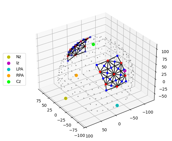
The location of the probes is obtained from the snirf metadata.

The units (‘mm’) are adopted and the coordinate system is named ‘digitized’.

[7]:

display(rec.geo3d)
print(f"CRS='{rec.geo3d.points.crs}'")

<xarray.DataArray (label: 346, digitized: 3)> Size: 8kB
[mm] -77.82 15.68 23.17 -61.91 21.23 56.49 ... 14.23 -38.28 81.95 -0.678 -37.03
Coordinates:
    type     (label) object 3kB PointType.SOURCE ... PointType.LANDMARK
  * label    (label) <U6 8kB 'S1' 'S2' 'S3' 'S4' ... 'FFT10h' 'FT10h' 'FTT10h'
Dimensions without coordinates: digitized

CRS='digitized'

[8]:

cedalion.vis.anatomy.plot_montage3D(rec["amp"], rec.geo3d)

../../_images/examples_tutorial_5_image_reconstruction_13_0.png

Preprocessing

[9]:

rec["od"] = cedalion.nirs.cw.int2od(rec["amp"])
rec["od_tddr"] = motion.tddr(rec["od"])
rec["od_wavelet"] = motion.wavelet(rec["od_tddr"])

# see 2_tutorial_preprocessing.ipynb for channel selection
bad_channels = ['S13D26', 'S14D28']

rec["od_clean"] = rec["od_wavelet"].sel(channel=~rec["od"].channel.isin(['S13D26', 'S14D28']))

od_var = quality.measurement_variance(rec["od_clean"], calc_covariance=False)

rec["od_mean_subtracted"], global_comp = physio.global_component_subtract(
    rec["od_clean"], ts_weights=1 / od_var, k=0
)

rec["od_freqfiltered"] = rec["od_mean_subtracted"].cd.freq_filter(
    fmin=0.01, fmax=0.5, butter_order=4
)

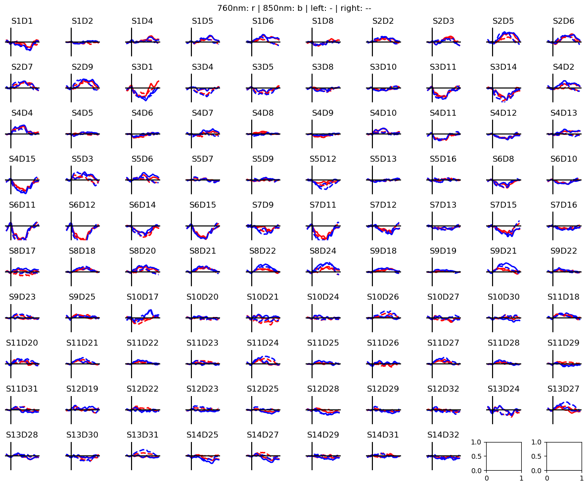
Calculate block averages in optical density

[10]:

# segment data into epochs
epochs = rec["od_freqfiltered"].cd.to_epochs(
        rec.stim, # stimulus dataframe
        ["FTapping/Left", "FTapping/Right"],  # select events, discard the others
        before=5 * cedalion.units.s, # seconds before stimulus
        after=30 * cedalion.units.s, # seconds after stimulus
)

# calculate baseline
baseline = epochs.sel(reltime=(epochs.reltime < 0)).mean("reltime")
# subtract baseline
epochs_blcorrected = epochs - baseline

# group trials by trial_type. For each group individually average the epoch dimension
blockaverage = epochs_blcorrected.groupby("trial_type").mean("epoch")

# Plot block averages. Please ignore errors if the plot is too small in the HD case

noPlts2 = int(np.ceil(np.sqrt(len(blockaverage.channel))))
f,ax = p.subplots(noPlts2,noPlts2, figsize=(12,10))
ax = ax.flatten()
for i_ch, ch in enumerate(blockaverage.channel):
    for ls, trial_type in zip(["-", "--"], blockaverage.trial_type):
        ax[i_ch].plot(blockaverage.reltime, blockaverage.sel(wavelength=760, trial_type=trial_type, channel=ch), "r", lw=2, ls=ls)
        ax[i_ch].plot(blockaverage.reltime, blockaverage.sel(wavelength=850, trial_type=trial_type, channel=ch), "b", lw=2, ls=ls)

    ax[i_ch].grid(1)
    ax[i_ch].set_title(ch.values)
    ax[i_ch].set_ylim(-.01, .01)
    ax[i_ch].set_axis_off()
    ax[i_ch].axhline(0, c="k")
    ax[i_ch].axvline(0, c="k")

p.suptitle("760nm: r | 850nm: b | left: - | right: --")
p.tight_layout()

../../_images/examples_tutorial_5_image_reconstruction_17_0.png

Constructing the TwoSurfaceHeadModel

See 1 - Head models and Forward Modelling for forther options to construct head models.

[11]:

if HEAD_MODEL in ["colin27", "icbm152"]:
    # use a factory method for the standard head models
    head_ijk = cedalion.dot.get_standard_headmodel(HEAD_MODEL)
else:
    raise ValueError("unknown head model")

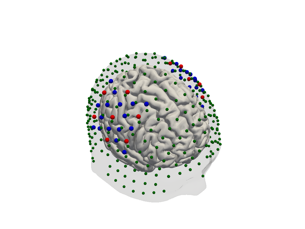
Optode Registration

The optode coordinates from the recording must be aligned with the scalp surface. A spring-relaxation algorithm is used to conform the montage to the scalp surface.

[12]:

geo3d_snapped_ijk, alignment_details = head_ijk.align_and_relax_to_scalp(rec.geo3d, rec["amp"])
display(geo3d_snapped_ijk)

<xarray.DataArray (label: 346, ijk: 3)> Size: 8kB
[] 14.82 141.3 98.21 30.84 146.4 129.8 ... 172.5 139.7 41.32 172.7 125.3 42.26
Coordinates:
    type     (label) object 3kB PointType.SOURCE ... PointType.LANDMARK
  * label    (label) <U6 8kB 'S1' 'S2' 'S3' 'S4' ... 'FFT10h' 'FT10h' 'FTT10h'
Dimensions without coordinates: ijk

[13]:

plt = pv.Plotter()
vbx.plot_surface(plt, head_ijk.brain, color="w")
vbx.plot_surface(plt, head_ijk.scalp, opacity=.1)
vbx.plot_labeled_points(plt, geo3d_snapped_ijk)
plt.show()

../../_images/examples_tutorial_5_image_reconstruction_22_0.png

[14]:

# remove landmarks from geo3d for subsequent plots
geo3d_plot = geo3d_snapped_ijk[geo3d_snapped_ijk.type != cdc.PointType.LANDMARK]

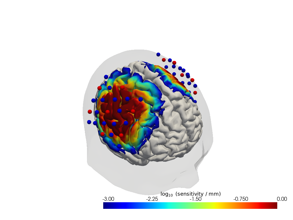
Sensitivity matrix

[15]:

Adot = cedalion.data.get_precomputed_sensitivity(DATASET, HEAD_MODEL)

Plot Sensitivity Matrix

[16]:

plotter = cedalion.vis.anatomy.sensitivity_matrix.Main(
    sensitivity=Adot,
    brain_surface=head_ijk.brain,
    head_surface=head_ijk.scalp,
    labeled_points=geo3d_plot,
)
plotter.plot(high_th=0, low_th=-3)
plotter.plt.show()

../../_images/examples_tutorial_5_image_reconstruction_27_0.png

Run the image reconstruction

The class cedalion.dot.ImageRecon implements several methods to solve the inverse problem of reconstructing activations in brain and scalp tissue that would explain the measured optical density changes in channel space.

[17]:

recon = cedalion.dot.ImageRecon(
    Adot,
    recon_mode="mua2conc",
    brain_only=False,
    alpha_meas=0.01,
    alpha_spatial=None,
    apply_c_meas=False,
    spatial_basis_functions=None,
)

In this example the channel-space block averages should be reconstructed into image space:

[18]:

blockaverage

Run the reconstruction and display results. Note how the OD time series with dimensions ('channel', 'wavelength', ...) transformed into a concentration time series with dimensions ('chromo', 'vertex', ...). The other dimensions ('trial_type', 'reltime') did not change.

The 'vertex' dimension has two coordinates:

is_brain: a boolean mask that discriminates between vertices on the brain and scalp surfaces
parcel: a string label attributed to each vertex according to a brain parcellation scheme (see section ‘Parcel Space’)

[19]:

img = recon.reconstruct(blockaverage)
img

[19]:

<xarray.DataArray (chromo: 2, vertex: 35050, trial_type: 2, reltime: 154)> Size: 173MB
[µM] -1.653e-13 -1.538e-13 -1.424e-13 ... -1.305e-12 -1.305e-12 -1.28e-12
Coordinates:
  * chromo      (chromo) <U3 24B 'HbO' 'HbR'
    parcel      (vertex) object 280kB 'VisCent_ExStr_8_LH' ... 'scalp'
    is_brain    (vertex) bool 35kB True True True True ... False False False
  * reltime     (reltime) float64 1kB -5.038 -4.809 -4.58 ... 29.54 29.77 30.0
  * trial_type  (trial_type) object 16B 'FTapping/Left' 'FTapping/Right'
Dimensions without coordinates: vertex

Visualizing image reconstruction results

In the following, different cedalion plot functions will be showcased to visualize concentration changes on the brain and scalp surfaces.

Channel Space

The function cedalion.vis.anatomy.scalp_plot_gif allows to create an animated gif of channel-space OD changes projected on the scalp.

Here, it is used to show the time course of the blockaveraged OD changes.

[20]:

# configure the plot
data_ts = blockaverage.sel(wavelength=850, trial_type="FTapping/Right")
# scalp_plot_gif expects the time dimension to be named 'time'
data_ts = data_ts.rename({"reltime": "time"})
filename_scalp = "scalp_plot_ts"

# call plot function
cedalion.vis.anatomy.scalp_plot_gif(
    data_ts,
    rec.geo3d,
    filename=filename_scalp,
    time_range=(-5, 30, 0.5) * units.s,
    scl=(-0.01, 0.01),
    fps=6,
    optode_size=6,
    optode_labels=True,
    str_title="OD 850 nm",
)

[21]:

display_image(f"{filename_scalp}.gif")

../../_images/examples_tutorial_5_image_reconstruction_37_0.png

Image Space

Single-View Animations of Activitations on the Brain

The function cedalion.vis.anatomy.image_recon_view allows to create an animated gif of image-space concentration changes projected on the brain.

[22]:

filename_view = 'image_recon_view'

# image_recon_view expects input with dimensions
# ("vertex", "chromo", "time") (in that order)
X_ts = img.sel(trial_type="FTapping/Right").rename({"reltime": "time"})
X_ts = X_ts.transpose("vertex", "chromo", "time")

scl = np.percentile(np.abs(X_ts.sel(chromo='HbO')).pint.dequantify(), 99)
clim = (-scl,scl)

cedalion.vis.anatomy.image_recon_view(
    X_ts,  # time series data; can be 2D (static) or 3D (dynamic)
    head_ijk,
    cmap='seismic',
    clim=clim,
    view_type='hbo_brain',
    view_position='left',
    title_str='HbO / µM',
    filename=filename_view,
    SAVE=True,
    time_range=(-5,30,0.5)*units.s,
    fps=6,
    geo3d_plot = geo3d_plot,
    wdw_size = (1024, 768)
)

[23]:

display_image(f"{filename_view}.gif")

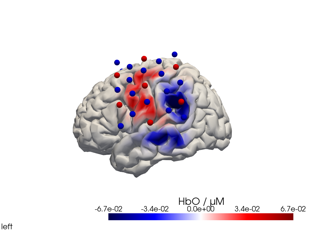
../../_images/examples_tutorial_5_image_reconstruction_40_0.png

Alternatively, we can just select a single time point and plot activity as a still image at that time. Note the different file suffix (.png).

[24]:

# selects the nearest time sample at t=4s in X_ts
# note: sel does not accept quantified units
X_ts_plot = X_ts.sel(time=4, method="nearest")

filename_view = 'image_recon_view_still'

cedalion.vis.anatomy.image_recon_view(
    X_ts_plot,  # time series data; can be 2D (static) or 3D (dynamic)
    head_ijk,
    cmap='seismic',
    clim=clim,
    view_type='hbo_brain',
    view_position='left',
    title_str='HbO / µM',
    filename=filename_view,
    SAVE=True,
    time_range=(-5,30,0.5)*units.s,
    fps=6,
    geo3d_plot = geo3d_plot,
    wdw_size = (1024, 768)
)

../../_images/examples_tutorial_5_image_reconstruction_42_0.png

[25]:

display_image(f"{filename_view}.png")

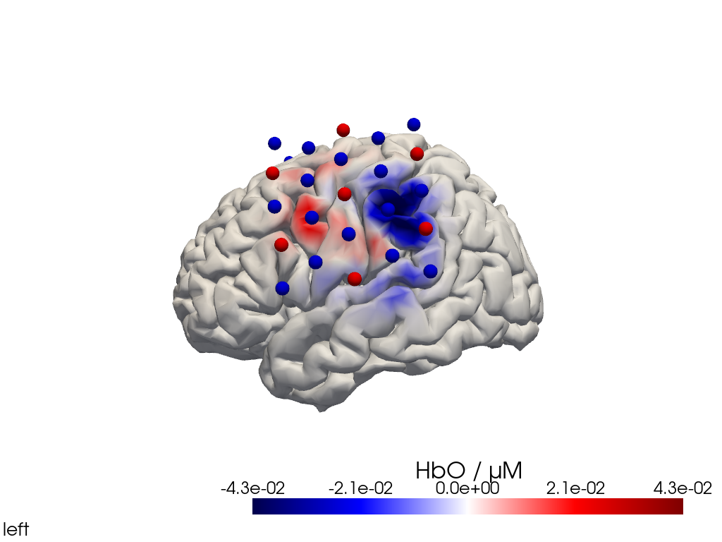
../../_images/examples_tutorial_5_image_reconstruction_43_0.png

Multi-View Animations of Activitations on the Brain

The function cedalion.vis.anatomy.image_recon_multi_view shows the activity on the brain from all angles as still image or animated across time:

[26]:

filename_multiview = 'image_recon_multiview'

# prepare data
X_ts = img.sel(trial_type="FTapping/Right").rename({"reltime": "time"})
X_ts = X_ts.transpose("vertex", "chromo", "time")

scl = np.percentile(np.abs(X_ts.sel(chromo='HbO')).pint.dequantify(), 99)
clim = (-scl,scl)

cedalion.vis.anatomy.image_recon_multi_view(
    X_ts,  # time series data; can be 2D (static) or 3D (dynamic)
    head_ijk,
    cmap='seismic',
    clim=clim,
    view_type='hbo_brain',
    title_str='HbO / µM',
    filename=filename_multiview,
    SAVE=True,
    time_range=(-5,30,0.5)*units.s,
    fps=6,
    geo3d_plot = None, #  geo3d_plot
    wdw_size = (1024, 768)
)

[27]:

display_image(f"{filename_multiview}.gif")

../../_images/examples_tutorial_5_image_reconstruction_46_0.png

Multi-View Animations of Activitations on the Scalp

This gives us activity on the scalp after recon from all angles as still image or across time

[28]:

filename_multiview_scalp = 'image_recon_multiview_scalp'

# prepare data
X_ts = img.sel(trial_type="FTapping/Right").rename({"reltime": "time"})
X_ts = X_ts.transpose("vertex", "chromo", "time")

scl = np.percentile(np.abs(X_ts.sel(chromo='HbO')).pint.dequantify(), 99)
clim = (-scl,scl)

cedalion.vis.anatomy.image_recon_multi_view(
    X_ts,  # time series data; can be 2D (static) or 3D (dynamic)
    head_ijk,
    cmap='seismic',
    clim=clim,
    view_type='hbo_scalp',
    title_str='HbO / uM',
    filename=filename_multiview_scalp,
    SAVE=True,
    time_range=(-5,30,0.5)*units.s,
    fps=6,
    geo3d_plot = geo3d_plot,
    wdw_size = (1024, 768)
)

[29]:

display_image(f"{filename_multiview_scalp}.gif")

../../_images/examples_tutorial_5_image_reconstruction_49_0.png

Parcel Space

The Schaefer Atlas [SKG+18] as implemented in Cedalion provides nearly 600 labels for different regions of the brain. Each vertex of the brain surface has its correspondng parcel label assigned as a coordinate.

[30]:

head_ijk.brain.vertices

[30]:

<xarray.DataArray (label: 25000, ijk: 3)> Size: 600kB
[] 82.52 19.84 68.31 83.52 20.32 65.89 ... 96.28 105.3 86.73 127.6 34.46 60.38
Coordinates:
  * label             (label) int64 200kB 0 1 2 3 4 ... 24996 24997 24998 24999
  * fsaverage_vertex  (label) int64 200kB 42 61 75 89 ... 333018 333020 333066
  * parcel            (label) object 200kB 'VisCent_ExStr_8_LH' ... 'VisCent_...
  * mni152_r          (label) float64 200kB -6.792 -5.846 -10.87 ... 6.633 37.95
  * mni152_a          (label) float64 200kB -104.8 -104.3 ... -19.16 -89.49
  * mni152_s          (label) float64 200kB -1.408 -3.845 ... 15.99 -10.04
Dimensions without coordinates: ijk

To obtain the average hemodynamic response in a parcel, the baseline-subtraced concentration changes of all vertices in a parcel are averaged. As baseline the first sample is used.

[31]:

# only consider brain vertices in the following.
img_brain = img.sel(vertex=img.is_brain)

# use the first sample along the reltime dimension as baseline
baseline =  img_brain.isel(reltime=0)
img_brain_blsubtracted = img_brain - baseline

display(img_brain_blsubtracted.rename("img_brain_blsubtracted"))

<xarray.DataArray 'img_brain_blsubtracted' (chromo: 2, vertex: 25000,
                                            trial_type: 2, reltime: 154)> Size: 123MB
[µM] 0.0 1.158e-14 2.29e-14 3.571e-14 ... -3.329e-12 -3.24e-12 -3.051e-12
Coordinates:
  * chromo      (chromo) <U3 24B 'HbO' 'HbR'
    parcel      (vertex) object 200kB 'VisCent_ExStr_8_LH' ... 'VisCent_ExStr...
    is_brain    (vertex) bool 25kB True True True True ... True True True True
  * reltime     (reltime) float64 1kB -5.038 -4.809 -4.58 ... 29.54 29.77 30.0
  * trial_type  (trial_type) object 16B 'FTapping/Left' 'FTapping/Right'
Dimensions without coordinates: vertex

Using parcel labels, vertices belonging to the same brain region can be easily grouped together with the DataArray.groupby function. On these vertex groups many reduction methods can be executed. He we use the function mean() to average over vertices.

Note how the time series dimension changed from vertex to parcel:

[32]:

# average over parcels
avg_HbO = img_brain_blsubtracted.sel(chromo="HbO").groupby('parcel').mean()
avg_HbR = img_brain_blsubtracted.sel(chromo="HbR").groupby('parcel').mean()

display(avg_HbO.rename("avg_HbO"))

<xarray.DataArray 'avg_HbO' (parcel: 601, trial_type: 2, reltime: 154)> Size: 1MB
[µM] 0.0 4.521e-11 1.252e-10 2.449e-10 ... -1.266e-13 -1.245e-13 -1.249e-13
Coordinates:
    chromo      <U3 12B 'HbO'
  * reltime     (reltime) float64 1kB -5.038 -4.809 -4.58 ... 29.54 29.77 30.0
  * trial_type  (trial_type) object 16B 'FTapping/Left' 'FTapping/Right'
  * parcel      (parcel) object 5kB 'Background+FreeSurfer_Defined_Medial_Wal...

The montage in this dataset covers only parts of the head. Consequently, many brain regions lack significant signal coverage due to the absence of optodes.

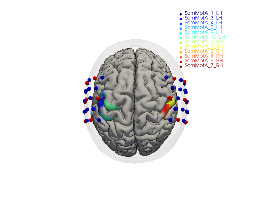
To focus on relevant regions, a subset of parcels from the somatosensory and motor regions in both hemispheres is selected.

[33]:

selected_parcels = [
    "SomMotA_1_LH", "SomMotA_3_LH", "SomMotA_4_LH",
    "SomMotA_5_LH", "SomMotA_9_LH", "SomMotA_10_LH",

    "SomMotA_1_RH", "SomMotA_2_RH", "SomMotA_3_RH",
    "SomMotA_4_RH", "SomMotA_6_RH", "SomMotA_7_RH"
]

The following plot visualizes the montage and the selected parcels:

[34]:

# map parcel labels to colors
parcel_colors = {
    parcel: p.cm.jet(i / (len(selected_parcels) - 1))
    for i, parcel in enumerate(selected_parcels)
}

plt = pv.Plotter()

vbx.plot_surface(
    plt,
    head_ijk.scalp,
    color="w",
    opacity=.1
)

vbx.plot_surface(
    plt,
    head_ijk.brain,
    color=np.asarray(
        [
            parcel_colors.get(parcel, (0.8, 0.8, 0.8, 1.))
            for parcel in head_ijk.brain.vertices.parcel.values
        ]
    ),
    silhouette=True,
)

vbx.plot_labeled_points(plt, geo3d_plot)

plt.add_legend(labels=parcel_colors.items(), face="o", size=(0.3, 0.3))

vbx.camera_at_cog(plt, head_ijk.brain, rpos=(0, 0, 1), up=(0, 1, 0), fit_scene=True)
plt.show()

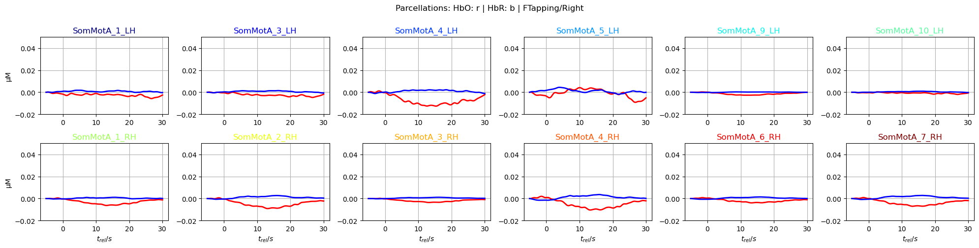
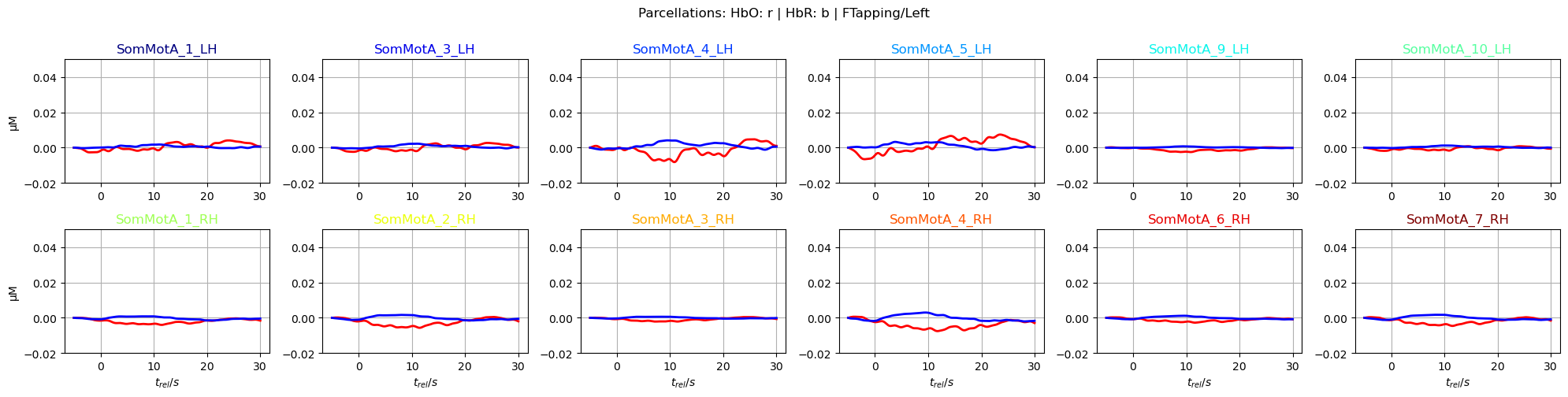
../../_images/examples_tutorial_5_image_reconstruction_59_0.png

Plot averaged time traces in each parcel for the ‘FTapping/Right’ and ‘FTapping/Left’ conditions:

[35]:

f,ax = p.subplots(2,6, figsize=(20,5))
ylims = -0.02, 0.05
ax = ax.flatten()
for i_par, par in enumerate(selected_parcels):
    ax[i_par].plot(avg_HbO.sel(parcel = par, trial_type = "FTapping/Right").reltime, avg_HbO.sel(parcel = par, trial_type = "FTapping/Right"), "r", lw=2, ls='-')
    ax[i_par].plot(avg_HbR.sel(parcel = par, trial_type = "FTapping/Right").reltime, avg_HbR.sel(parcel = par, trial_type = "FTapping/Right"), "b", lw=2, ls='-')

    ax[i_par].grid(1)
    ax[i_par].set_title(par, color=parcel_colors[par])
    ax[i_par].set_ylim(*ylims)

    if i_par % 6 == 0:
        ax[i_par].set_ylabel("µM")
    if i_par >=6:
        ax[i_par].set_xlabel("$t_{rel} / s$")

p.suptitle("Parcellations: HbO: r | HbR: b | FTapping/Right", y=1)
p.tight_layout()

f,ax = p.subplots(2,6, figsize=(20,5))
ax = ax.flatten()
for i_par, par in enumerate(selected_parcels):
    ax[i_par].plot(avg_HbO.sel(parcel = par, trial_type = "FTapping/Left").reltime, avg_HbO.sel(parcel = par, trial_type = "FTapping/Left"), "r", lw=2, ls='-')
    ax[i_par].plot(avg_HbR.sel(parcel = par, trial_type = "FTapping/Left").reltime, avg_HbR.sel(parcel = par, trial_type = "FTapping/Left"), "b", lw=2, ls='-')

    ax[i_par].grid(1)
    ax[i_par].set_title(par, color=parcel_colors[par])
    ax[i_par].set_ylim(*ylims)

    if i_par % 6 == 0:
        ax[i_par].set_ylabel("µM")
    if i_par >=6:
        ax[i_par].set_xlabel("$t_{rel} / s$")

p.suptitle("Parcellations: HbO: r | HbR: b | FTapping/Left", y=1)
p.tight_layout()

../../_images/examples_tutorial_5_image_reconstruction_61_0.png

../../_images/examples_tutorial_5_image_reconstruction_61_1.png

References

[36]:

cedalion.bib.dump_to_notebook()

Methods used

[1]	Tucker2022	cedalion.io.snirf.read_snirf	Stephen Tucker, Jay Dubb, Sreekanth Kura, Alexander von Lühmann, Robert Franke, Jörn M. Horschig, Samuel Powell, Robert Oostenveld, Michael Lührs, Édouard Delaire, Zahra M. Aghajan, Hanseok Yun, Meryem A. Yücel, Qianqian Fang, Theodore J. Huppert, Blaise deB. Frederick, Luca Pollonini, David A. Boas, and Robert Luke. Introduction to the shared near infrared spectroscopy format. Neurophotonics, 10(1):013507, 2022. doi:10.1117/1.NPh.10.1.013507.
[2]	Delpy1988	cedalion.nirs.cw.int2od	D. T. Delpy, M. Cope, P. van der Zee, S. Arridge, S. Wray, and J. Wyatt. Estimation of optical pathlength through tissue from direct time of flight measurement. Physics in Medicine and Biology, 33(12):1433–1442, 1988. doi:10.1088/0031-9155/33/12/008.
[3]	Villringer1997	cedalion.nirs.cw.int2od	Arno Villringer and Britton Chance. Non-invasive optical spectroscopy and imaging of human brain function. Trends in Neurosciences, 20(10):435–442, 1997. doi:10.1016/S0166-2236(97)01132-6.
[4]	Fishburn2019	cedalion.sigproc.motion.tddr	Frank A. Fishburn, Ruth S. Ludlum, Chandan J. Vaidya, and Andrei V. Medvedev. Temporal derivative distribution repair (tddr): a motion correction method for fnirs. NeuroImage, 184:171–179, 2019. doi:https://doi.org/10.1016/j.neuroimage.2018.09.025.
[5]	Fishburn2018	cedalion.sigproc.motion.tddr	Frank Fishburn. Tddr. 2018. URL: https://github.com/frankfishburn/TDDR/.
[6]	Molavi2012	cedalion.sigproc.motion.wavelet	Behnam Molavi and Guy A Dumont. Wavelet-based motion artifact removal for functional near-infrared spectroscopy. Physiological Measurement, 33(2):259, 2012. doi:10.1088/0967-3334/33/2/259.
[7]	Huppert2009	cedalion.sigproc.motion.wavelet	Theodore J. Huppert, Solomon G. Diamond, Maria A. Franceschini, and David A. Boas. Homer: a review of time-series analysis methods for near-infrared spectroscopy of the brain. Appl. Opt., 48(10):D280–D298, Apr 2009. doi:https://doi.org/10.1364/AO.48.00D280.
[8]	Holmes1998	cedalion.data.get_colin27_headmodel_files	Colin J. Holmes, Rick Hoge, Louis Collins, Roger Woods, Arthur W. Toga, and Alan C. Evans. Enhancement of mr images using registration for signal averaging. Journal of Computer Assisted Tomography, 22(2):324–333, March 1998. doi:10.1097/00004728-199803000-00032.
[9]	Fischl2012	cedalion.data.get_colin27_headmodel_files	Bruce Fischl. FreeSurfer. NeuroImage, 62(2):774–781, 2012. doi:10.1016/j.neuroimage.2012.01.021.
[10]	Schaefer2018	cedalion.data.get_colin27_headmodel_files	Alexander Schaefer, Ru Kong, Evan M Gordon, Timothy O Laumann, Xi-Nian Zuo, Avram J Holmes, Simon B Eickhoff, and BT Thomas Yeo. Local-global parcellation of the human cerebral cortex from intrinsic functional connectivity mri. Cerebral cortex, 28(9):3095–3114, 2018. doi:10.1093/cercor/bhx179.
[11]	Aasted2015	cedalion.dot.head_model.TwoSurfaceHeadModel.align_and_relax_to_scalp	Christopher M. Aasted, Meryem A. Yücel, Robert J. Cooper, Jay Dubb, Daisuke Tsuzuki, Lino Becerra, Martin P. Petkov, David Borsook, Ippeita Dan, and David A. Boas. Anatomical guidance for functional near-infrared spectroscopy: AtlasViewer tutorial. Neurophotonics, 2(2):020801, 2015. doi:10.1117/1.NPh.2.2.020801.
[12]	Fang2009	cedalion.data.get_precomputed_sensitivity	Qianqian Fang and David A Boas. Monte carlo simulation of photon migration in 3d turbid media accelerated by graphics processing units. Optics express, 17(22):20178–20190, 2009. doi:10.1364/OE.17.020178.
[13]	Yu2018	cedalion.data.get_precomputed_sensitivity	Leiming Yu, Fanny Nina-Paravecino, David Kaeli, and Qianqian Fang. Scalable and massively parallel monte carlo photon transport simulations for heterogeneous computing platforms. Journal of biomedical optics, 23(1):010504–010504, 2018. doi:10.1117/1.JBO.23.1.010504.
[14]	Yan2020	cedalion.data.get_precomputed_sensitivity	Shijie Yan and Qianqian Fang. Hybrid mesh and voxel based monte carlo algorithm for accurate and efficient photon transport modeling in complex bio-tissues. Biomedical Optics Express, 11(11):6262–6270, 2020. doi:10.1364/BOE.409468.
[15]	Carlton2026	cedalion.dot.image_recon.ImageRecon.__init__	Laura B. Carlton, Miray Altınkaynak, Shannon Kelley, Bernhard B. Zimmermann, Sreekanth Kura, Eike Middell, Alexander von Lühmann, Emily P. Stephen, Meryem A. Yücel, and David A. Boas. Surface-based image reconstruction optimization for high-density functional near-infrared spectroscopy. Neurophotonics, 13(2):025001, 2026. doi:10.1117/1.NPh.13.2.025001.
[16]	Markow2025	cedalion.dot.image_recon.ImageRecon.__init__	Zachary E. Markow, Jason W. Trobaugh, Edward J. Richter, Kalyan Tripathy, Sean M. Rafferty, Alexandra M. Svoboda, Mariel L. Schroeder, Tracy M. Burns-Yocum, Karla M. Bergonzi, Mark A. Chevillet, Emily M. Mugler, Adam T. Eggebrecht, and Joseph P. Culver. Ultra high density imaging arrays in diffuse optical tomography for human brain mapping improve image quality and decoding performance. Scientific Reports, 15(1):3175, January 2025. doi:10.1038/s41598-025-85858-7.
[17]	Prahl1998	cedalion.nirs.common.get_extinction_coefficients	Scott A. Prahl. Optical absorption of hemoglobin. Oregon Medical Laser Center, online resource, 1998. URL: https://omlc.org/spectra/hemoglobin/.

Next: 6 — Data-driven Analysis — unsupervised decomposition.

Magnitude	[[-77.817871 15.680613999999998 23.172269999999997] [-61.906841 21.227732000000003 56.492802] [-85.37146 -16.079958 8.900885] ... [77.521 28.883 -39.113] [80.59 14.229 -38.278] [81.95 -0.678 -37.027]]
Units	millimeter

Magnitude	[[82.522325 19.841515 68.313221] [83.516588 20.319351 65.886337] [78.524571 20.543388 63.648142] ... [127.025612 152.660339 99.546274] [96.280465 105.252083 86.734898] [127.619801 34.463676 60.37505]]
Units	dimensionless