Assigning AAL3 and Brodmann Atlas Labels to Brain Surfaces

This notebook assigns AAL3 and Brodmann atlas labels to the Colin27 and ICBM152 brain surfaces, visualizes the labels, and summarizes their overlap with the Schaefer2018 parcels.

Overview

Neuroimaging atlases — parcellations that divide the cerebral cortex into anatomically or functionally defined regions — are a cornerstone of group-level fNIRS and DOT analysis. Atlases allow researchers to:

• Report results in a standardised anatomical vocabulary that is comparable across studies and laboratories.

• Aggregate channel or vertex signals into region-of-interest (ROI) time series, reducing the multiple-comparisons burden.

• Cross-reference DOT activations with the large fMRI literature, where the same atlas labels are widely used.

MNI space as a shared coordinate system

Most brain atlases are defined and distributed in MNI (Montreal Neurological Institute) space: a standardised brain coordinate frame derived from averaging many individual MRI scans into a common template. Every standard head model in Cedalion — Colin27 [HHC+98] and ICBM152 [FEB+11] — carries pre-computed MNI152 coordinates for every brain surface vertex. This means that any volumetric atlas provided as a NIfTI file in MNI space can be transferred to the brain surface without any additional registration step: the shared coordinate system acts as the bridge between the volumetric atlas and the surface model.

The two MNI spaces: MNI152 and MNI305

Two MNI variants are in common use and it is important to keep them distinct:

Space	Template	Typical users
MNI152	Average of 152 adult brains (ICBM152 template)	FSL, recent SPM, most modern atlases
MNI305	Average of 305 brains; the original MNI reference	FreeSurfer, older SPM, some legacy atlases

MNI152 and MNI305 differ by a small affine shift (a few millimetres in some regions) and are not interchangeable. Cedalion stores a pre-computed affine transform (cedalion.dot.utils.mni305_to_mni152) and applies it automatically when a NIfTI is declared as voxel_label_crs='mni305', so you do not need to handle the conversion manually. Both spaces are fully supported; you simply specify which one your NIfTI file uses.

What this notebook demonstrates

This notebook shows the general workflow for applying any user-supplied parcellation scheme — provided as a NIfTI label volume in either MNI152 or MNI305 space — to the Cedalion head models. The workflow is illustrated with two widely used atlases:

• AAL3 (Automated Anatomical Labelling atlas, version 3) [RHL+20] — 170 macro-anatomical regions covering the entire cerebral cortex and subcortex.

• Brodmann areas (Mai–Majtanik atlas) [MM17] — the classical cytoarchitectonic map, available as a volumetric MNI label file.

Both atlases are bundled with Cedalion and loaded via cedalion.data.get_atlas_files(). The same code applies unchanged to any other NIfTI atlas you supply.

For more detail, see also:

• 43a_head_models_overview.ipynb — introduction to TwoSurfaceHeadModel and the Schaefer2018 parcellation bundled with the standard models

• 43b_individualized_head_models.ipynb — building an individualized head model from a subject’s own MRI using FreeSurfer, which yields surface-native parcel labels with sharper boundaries than the volumetric approach shown here

import json

import numpy as np
import pyvista as pv
from scipy.spatial import KDTree

import cedalion
import cedalion.dot
from cedalion.vis.anatomy import get_vertex_colors_from_coord, plot_brain_views_grid

pv.set_jupyter_backend("static")


def display_truncated_dict(d: dict):
    "Helper function for displaying long dictionaries."

    keys = list(d)[:5] + list(d)[-5:]
    display({k : d[k] for k in keys})

Loading Colin27 and ICBM152 Head Models

We load both standard atlas head models. Each is stored in voxel space (crs='ijk'); assign_parcels_via_mni_coords works in MNI152 space internally so the coordinate system of the loaded head model does not need to match that of the atlas.

Both models carry pre-computed mni152_r/a/s vertex coordinates on the brain surface, which is what makes the atlas transfer possible. The inflated cortex surfaces are loaded for visualization: inflation removes sulci and gyri so that buried cortex becomes visible, making parcel boundaries much easier to inspect.

colin_ijk = cedalion.dot.get_standard_headmodel("colin27")
colin_inflated = cedalion.dot.get_inflated_cortex_surface("colin27")

icbm_ijk = cedalion.dot.get_standard_headmodel("icbm152")
icbm_inflated = cedalion.dot.get_inflated_cortex_surface("icbm152")

Loading Atlases

Atlases distributed for use with standard MNI templates typically come in two files:

1. A NIfTI volume (.nii or .nii.gz) in which every voxel inside a labelled region carries a positive integer, and background voxels carry 0 (or another reserved value).

2. A label mapping (.json, .csv, or .txt) that translates those integers to human-readable region names.

cedalion.data.get_atlas_files(name) returns both paths for the bundled atlases. For a custom atlas you can pass any NIfTI path you have downloaded or created.

AAL3 — Automated Anatomical Labelling atlas (version 3)

AAL3 [RHL+20] divides the cerebral cortex and subcortical structures into 170 macro-anatomical regions based on sulcal and gyral landmarks visible in the MNI152 template. It is one of the most widely used atlases in the fMRI and fNIRS literature and provides a common vocabulary for reporting results. The NIfTI file bundled with Cedalion is defined in MNI152 space.

aal3_voxel_label_niftii, aal3_labels_json = cedalion.data.get_atlas_files("aal3")

# dictionary to map numeric voxel labels in nifti to string labels
with aal3_labels_json.open("r") as fin:
    aal3_num2label = json.load(fin)
    aal3_num2label = {i["index"] : i["name"] for i in aal3_num2label["labels"]}

# show some entries of the dictionary
display_truncated_dict((aal3_num2label))

Downloading file 'atlas_aal3.zip' from 'https://doc.ibs.tu-berlin.de/cedalion/datasets/dev/atlas_aal3.zip' to '/home/runner/.cache/cedalion/dev'.
Unzipping contents of '/home/runner/.cache/cedalion/dev/atlas_aal3.zip' to '/home/runner/.cache/cedalion/dev/atlas_aal3.zip.unzip'

{1: 'Precentral_L',
 2: 'Precentral_R',
 3: 'Frontal_Sup_2_L',
 4: 'Frontal_Sup_2_R',
 5: 'Frontal_Mid_2_L',
 166: 'Red_N_R',
 167: 'LC_L',
 168: 'LC_R',
 169: 'Raphe_D',
 170: 'Raphe_M'}

Brodmann Areas — Mai–Majtanik Atlas

Brodmann areas are the classical cytoarchitectonic map of the human cortex, originally defined by Korbinian Brodmann in 1909 from histological sections and still widely used to communicate the location of activations in the neuroscience literature. The Mai–Majtanik atlas [MM17] provides these areas as a digitised volumetric label map registered to MNI152 space, making it directly compatible with the Cedalion head models. Areas such as BA44/45 (Broca’s area) or BA17 (primary visual cortex) are convenient reference landmarks when linking fNIRS results to the broader neuroimaging literature.

brodmann_voxel_label_niftii, brodmann_labels_json = cedalion.data.get_atlas_files("brodmann")

# dictionary to map numeric voxel labels in nifti to string labels
with brodmann_labels_json.open("r") as fin:
    brodmann_num2label = json.load(fin)
    brodmann_num2label = {i["index"] : i["name"] for i in brodmann_num2label["labels"]}

# show some entries of the dictionary
display_truncated_dict(brodmann_num2label)

Downloading file 'atlas_brodmann.zip' from 'https://doc.ibs.tu-berlin.de/cedalion/datasets/dev/atlas_brodmann.zip' to '/home/runner/.cache/cedalion/dev'.
Unzipping contents of '/home/runner/.cache/cedalion/dev/atlas_brodmann.zip' to '/home/runner/.cache/cedalion/dev/atlas_brodmann.zip.unzip'

{1: 'right_Ent',
 2: 'right_BA20',
 3: 'right_BA38',
 4: 'right_BA21',
 5: 'right_BA36',
 139: 'left_BA8',
 140: 'left_BA5',
 141: 'left_BA52',
 142: 'left_BA35',
 143: 'left_BA34'}

Brain Vertex Coordinates Before Atlas Assignment

The brain.vertices xarray DataArray already carries several vertex coordinates set when the head model was built from FreeSurfer outputs:

Coordinate	Meaning
parcel	Schaefer2018 parcel label [SKG+18]
fsaverage_vertex	Corresponding vertex index in the FreeSurfer fsaverage template
mni152_r/a/s	MNI152 RAS coordinates of the vertex in mm

Calling assign_parcels_via_mni_coords will add a new named coordinate to this DataArray without removing or modifying any existing one. Multiple atlas labels can therefore coexist on the same vertex, which is what we exploit below.

colin_ijk.brain.vertices

<xarray.DataArray (label: 25000, ijk: 3)> Size: 600kB
<Quantity([[ 77.575966  19.290176  74.323414]
 [ 84.207517  19.202515  68.985718]
 [ 85.092731  19.342216  67.495901]
 ...
 [156.792999 124.600063  70.614239]
 [132.153282 182.175888  72.333395]
 [ 94.202573  52.128399 103.226031]], 'dimensionless')>
Coordinates:
  * label             (label) int64 200kB 0 1 2 3 4 ... 24996 24997 24998 24999
  * fsaverage_vertex  (label) int64 200kB 6 28 39 42 ... 333163 333191 333192
  * parcel            (label) object 200kB 'VisCent_ExStr_8_LH' ... 'VisPeri_...
  * mni152_r          (label) float64 200kB -11.62 -5.094 -4.239 ... 41.6 5.238
  * mni152_a          (label) float64 200kB -105.4 -105.4 -105.3 ... 58.39 -72.4
  * mni152_s          (label) float64 200kB 4.655 -0.753 -2.251 ... 0.446 32.95
Dimensions without coordinates: ijk

xarray.DataArray

• label: 25000
• ijk: 3

• [] 77.58 19.29 74.32 84.21 19.2 68.99 ... 182.2 72.33 94.2 52.13 103.2

  Magnitude	[[77.575966 19.290176 74.323414] [84.207517 19.202515 68.985718] [85.092731 19.342216 67.495901] ... [156.792999 124.600063 70.614239] [132.153282 182.175888 72.333395] [94.202573 52.128399 103.226031]]
  Units	dimensionless

• Coordinates: (6)
  • label
    (label)
    int64
    0 1 2 3 ... 24996 24997 24998 24999

    array([    0,     1,     2, ..., 24997, 24998, 24999], shape=(25000,))

  • fsaverage_vertex
    (label)
    int64
    6 28 39 42 ... 333163 333191 333192

    array([     6,     28,     39, ..., 333163, 333191, 333192], shape=(25000,))

  • parcel
    (label)
    object
    'VisCent_ExStr_8_LH' ... 'VisPer...

    array(['VisCent_ExStr_8_LH', 'VisCent_Striate_2_LH', 'VisCent_Striate_2_LH',
           ..., 'TempPar_1_RH', 'SalVentAttnB_PFClv_2_RH', 'VisPeri_ExStrSup_3_RH'],
          shape=(25000,), dtype=object)

  • mni152_r
    (label)
    float64
    -11.62 -5.094 -4.239 ... 41.6 5.238

    array([-11.616,  -5.094,  -4.239, ...,  66.569,  41.601,   5.238],
          shape=(25000,))

  • mni152_a
    (label)
    float64
    -105.4 -105.4 ... 58.39 -72.4

    array([-105.443, -105.421, -105.265, ...,    1.127,   58.391,  -72.402],
          shape=(25000,))

  • mni152_s
    (label)
    float64
    4.655 -0.753 -2.251 ... 0.446 32.95

    array([ 4.655, -0.753, -2.251, ..., -1.053,  0.446, 32.952], shape=(25000,))

• Indexes: (6)
  • label
    PandasIndex

    PandasIndex(Index([    0,     1,     2,     3,     4,     5,     6,     7,     8,     9,
           ...
           24990, 24991, 24992, 24993, 24994, 24995, 24996, 24997, 24998, 24999],
          dtype='int64', name='label', length=25000))

  • fsaverage_vertex
    PandasIndex

    PandasIndex(Index([     6,     28,     39,     42,     70,     79,     87,     88,     89,
               98,
           ...
           333023, 333032, 333063, 333124, 333138, 333155, 333162, 333163, 333191,
           333192],
          dtype='int64', name='fsaverage_vertex', length=25000))

  • parcel
    PandasIndex

    PandasIndex(Index(['VisCent_ExStr_8_LH', 'VisCent_Striate_2_LH', 'VisCent_Striate_2_LH',
           'VisCent_Striate_2_LH', 'VisCent_ExStr_8_LH', 'VisCent_ExStr_8_LH',
           'VisCent_ExStr_8_LH', 'VisCent_Striate_2_LH', 'VisCent_Striate_2_LH',
           'VisCent_ExStr_8_LH',
           ...
           'DefaultA_pCunPCC_7_RH', 'ContC_pCun_5_RH', 'TempPar_5_RH',
           'DefaultA_pCunPCC_6_RH', 'ContC_pCun_3_RH', 'VisPeri_ExStrSup_6_RH',
           'ContC_pCun_2_RH', 'TempPar_1_RH', 'SalVentAttnB_PFClv_2_RH',
           'VisPeri_ExStrSup_3_RH'],
          dtype='object', name='parcel', length=25000))

  • mni152_r
    PandasIndex

    PandasIndex(Index([-11.616,  -5.094,  -4.239,  -7.416, -12.264, -10.238, -11.554,  -5.342,
            -6.943,  -12.29,
           ...
              2.42,   10.23,   51.59,   4.062,   2.648,  25.361,  10.531,  66.569,
            41.601,   5.238],
          dtype='float64', name='mni152_r', length=25000))

  • mni152_a
    PandasIndex

    PandasIndex(Index([-105.443, -105.421, -105.265, -105.837, -105.464, -105.191, -104.527,
           -104.293, -104.573, -103.244,
           ...
            -15.904,  -72.945,  -32.605,  -25.785,  -41.791,  -76.709,  -77.473,
              1.127,   58.391,  -72.402],
          dtype='float64', name='mni152_a', length=25000))

  • mni152_s
    PandasIndex

    PandasIndex(Index([ 4.655, -0.753, -2.251, -1.384, -4.492, -5.601, -7.111,  8.289,  7.428,
            8.515,
           ...
           36.828, 47.624,  6.069, 53.443, 46.336, 40.184,  41.73, -1.053,  0.446,
           32.952],
          dtype='float64', name='mni152_s', length=25000))

• Attributes: (0)

Assigning Atlas Labels to Brain Vertices

TwoSurfaceHeadModel.assign_parcels_via_mni_coords transfers labels from a volumetric NIfTI atlas to the brain surface by exploiting the MNI152 coordinates shared by both. The algorithm works as follows:

1. Coordinate alignment: The NIfTI affine transform is used to compute the MNI coordinate of every voxel centre. If the atlas is in MNI305 space (voxel_label_crs='mni305'), the pre-computed affine cedalion.dot.utils.mni305_to_mni152 is applied first to bring voxel coordinates into the same MNI152 frame as the head model vertices.

2. Nearest-labelled-voxel search: A KD-tree is built from the voxel centres. For each brain surface vertex, all voxels within a ball of radius mni_eps mm in MNI152 space are retrieved. Background voxels (label 0 or whichever integer maps to background_label) are excluded, and the closest labelled voxel is selected.

3. Label assignment: The integer label of the winning voxel is translated to a string via label_mapping and stored as a new vertex coordinate. If no labelled voxel falls within mni_eps mm, the vertex receives background_label.

Key parameters:

Parameter	Effect
coordinate_label	Name of the new vertex coordinate (e.g. 'parcel_aal3')
label_mapping	{int: str} dict mapping numeric voxel labels to region names
voxel_label_niftii	Path to the NIfTI atlas file
voxel_label_crs	MNI variant of the NIfTI: 'mni152' (default) or 'mni305'
mni_eps	Search radius in mm (default 5). Increase if many vertices receive 'Background'

Each call returns a new head model object; the original is not modified (immutable-style API). We chain two calls to assign both atlases in sequence.

Assigning AAL3 and Brodmann labels to the Colin27 head:

# Colin27

colin_ijk_labeled = colin_ijk.assign_parcels_via_mni_coords(
    coordinate_label="parcel_aal3",
    label_mapping=aal3_num2label,
    voxel_label_niftii=aal3_voxel_label_niftii,
    voxel_label_crs="mni152",
    mni_eps=5
)

colin_ijk_labeled = colin_ijk_labeled.assign_parcels_via_mni_coords(
    coordinate_label="parcel_brodmann",
    label_mapping=brodmann_num2label,
    voxel_label_niftii=brodmann_voxel_label_niftii,
    voxel_label_crs="mni152",
    mni_eps=5
)


colin_ijk_labeled.brain.vertices

<xarray.DataArray (label: 25000, ijk: 3)> Size: 600kB
<Quantity([[ 77.575966  19.290176  74.323414]
 [ 84.207517  19.202515  68.985718]
 [ 85.092731  19.342216  67.495901]
 ...
 [156.792999 124.600063  70.614239]
 [132.153282 182.175888  72.333395]
 [ 94.202573  52.128399 103.226031]], 'dimensionless')>
Coordinates:
  * label             (label) int64 200kB 0 1 2 3 4 ... 24996 24997 24998 24999
  * fsaverage_vertex  (label) int64 200kB 6 28 39 42 ... 333163 333191 333192
  * parcel            (label) object 200kB 'VisCent_ExStr_8_LH' ... 'VisPeri_...
  * mni152_r          (label) float64 200kB -11.62 -5.094 -4.239 ... 41.6 5.238
  * mni152_a          (label) float64 200kB -105.4 -105.4 -105.3 ... 58.39 -72.4
  * mni152_s          (label) float64 200kB 4.655 -0.753 -2.251 ... 0.446 32.95
  * parcel_aal3       (label) <U20 2MB 'Occipital_Mid_L' ... 'Cuneus_R'
  * parcel_brodmann   (label) <U10 1MB 'left_BA17' 'left_BA17' ... 'right_BA19'
Dimensions without coordinates: ijk

xarray.DataArray

• label: 25000
• ijk: 3

• [] 77.58 19.29 74.32 84.21 19.2 68.99 ... 182.2 72.33 94.2 52.13 103.2

  Magnitude	[[77.575966 19.290176 74.323414] [84.207517 19.202515 68.985718] [85.092731 19.342216 67.495901] ... [156.792999 124.600063 70.614239] [132.153282 182.175888 72.333395] [94.202573 52.128399 103.226031]]
  Units	dimensionless

• Coordinates: (8)
  • label
    (label)
    int64
    0 1 2 3 ... 24996 24997 24998 24999

    array([    0,     1,     2, ..., 24997, 24998, 24999], shape=(25000,))

  • fsaverage_vertex
    (label)
    int64
    6 28 39 42 ... 333163 333191 333192

    array([     6,     28,     39, ..., 333163, 333191, 333192], shape=(25000,))

  • parcel
    (label)
    object
    'VisCent_ExStr_8_LH' ... 'VisPer...

    array(['VisCent_ExStr_8_LH', 'VisCent_Striate_2_LH', 'VisCent_Striate_2_LH',
           ..., 'TempPar_1_RH', 'SalVentAttnB_PFClv_2_RH', 'VisPeri_ExStrSup_3_RH'],
          shape=(25000,), dtype=object)

  • mni152_r
    (label)
    float64
    -11.62 -5.094 -4.239 ... 41.6 5.238

    array([-11.616,  -5.094,  -4.239, ...,  66.569,  41.601,   5.238],
          shape=(25000,))

  • mni152_a
    (label)
    float64
    -105.4 -105.4 ... 58.39 -72.4

    array([-105.443, -105.421, -105.265, ...,    1.127,   58.391,  -72.402],
          shape=(25000,))

  • mni152_s
    (label)
    float64
    4.655 -0.753 -2.251 ... 0.446 32.95

    array([ 4.655, -0.753, -2.251, ..., -1.053,  0.446, 32.952], shape=(25000,))

  • parcel_aal3
    (label)
    <U20
    'Occipital_Mid_L' ... 'Cuneus_R'

    array(['Occipital_Mid_L', 'Calcarine_L', 'Calcarine_L', ...,
           'Temporal_Pole_Sup_R', 'Frontal_Mid_2_R', 'Cuneus_R'],
          shape=(25000,), dtype='<U20')

  • parcel_brodmann
    (label)
    <U10
    'left_BA17' ... 'right_BA19'

    array(['left_BA17', 'left_BA17', 'left_BA17', ..., 'right_BA22', 'right_BA46',
           'right_BA19'], shape=(25000,), dtype='<U10')

• Indexes: (8)
  • label
    PandasIndex

    PandasIndex(Index([    0,     1,     2,     3,     4,     5,     6,     7,     8,     9,
           ...
           24990, 24991, 24992, 24993, 24994, 24995, 24996, 24997, 24998, 24999],
          dtype='int64', name='label', length=25000))

  • fsaverage_vertex
    PandasIndex

    PandasIndex(Index([     6,     28,     39,     42,     70,     79,     87,     88,     89,
               98,
           ...
           333023, 333032, 333063, 333124, 333138, 333155, 333162, 333163, 333191,
           333192],
          dtype='int64', name='fsaverage_vertex', length=25000))

  • parcel
    PandasIndex

    PandasIndex(Index(['VisCent_ExStr_8_LH', 'VisCent_Striate_2_LH', 'VisCent_Striate_2_LH',
           'VisCent_Striate_2_LH', 'VisCent_ExStr_8_LH', 'VisCent_ExStr_8_LH',
           'VisCent_ExStr_8_LH', 'VisCent_Striate_2_LH', 'VisCent_Striate_2_LH',
           'VisCent_ExStr_8_LH',
           ...
           'DefaultA_pCunPCC_7_RH', 'ContC_pCun_5_RH', 'TempPar_5_RH',
           'DefaultA_pCunPCC_6_RH', 'ContC_pCun_3_RH', 'VisPeri_ExStrSup_6_RH',
           'ContC_pCun_2_RH', 'TempPar_1_RH', 'SalVentAttnB_PFClv_2_RH',
           'VisPeri_ExStrSup_3_RH'],
          dtype='object', name='parcel', length=25000))

  • mni152_r
    PandasIndex

    PandasIndex(Index([-11.616,  -5.094,  -4.239,  -7.416, -12.264, -10.238, -11.554,  -5.342,
            -6.943,  -12.29,
           ...
              2.42,   10.23,   51.59,   4.062,   2.648,  25.361,  10.531,  66.569,
            41.601,   5.238],
          dtype='float64', name='mni152_r', length=25000))

  • mni152_a
    PandasIndex

    PandasIndex(Index([-105.443, -105.421, -105.265, -105.837, -105.464, -105.191, -104.527,
           -104.293, -104.573, -103.244,
           ...
            -15.904,  -72.945,  -32.605,  -25.785,  -41.791,  -76.709,  -77.473,
              1.127,   58.391,  -72.402],
          dtype='float64', name='mni152_a', length=25000))

  • mni152_s
    PandasIndex

    PandasIndex(Index([ 4.655, -0.753, -2.251, -1.384, -4.492, -5.601, -7.111,  8.289,  7.428,
            8.515,
           ...
           36.828, 47.624,  6.069, 53.443, 46.336, 40.184,  41.73, -1.053,  0.446,
           32.952],
          dtype='float64', name='mni152_s', length=25000))

  • parcel_aal3
    PandasIndex

    PandasIndex(Index(['Occipital_Mid_L', 'Calcarine_L', 'Calcarine_L', 'Calcarine_L',
           'Calcarine_L', 'Calcarine_L', 'Calcarine_L', 'Calcarine_L',
           'Occipital_Sup_L', 'Occipital_Mid_L',
           ...
           'Cingulate_Mid_R', 'Precuneus_R', 'Temporal_Sup_R', 'Supp_Motor_Area_R',
           'Precuneus_R', 'Occipital_Sup_R', 'Cuneus_R', 'Temporal_Pole_Sup_R',
           'Frontal_Mid_2_R', 'Cuneus_R'],
          dtype='object', name='parcel_aal3', length=25000))

  • parcel_brodmann
    PandasIndex

    PandasIndex(Index(['left_BA17', 'left_BA17', 'left_BA17', 'left_BA17', 'left_BA17',
           'left_BA17', 'left_BA17', 'left_BA18', 'left_BA18', 'left_BA18',
           ...
           'right_BA23', 'right_BA7', 'right_BA22', 'right_BA4', 'right_BA31',
           'right_BA7', 'right_BA19', 'right_BA22', 'right_BA46', 'right_BA19'],
          dtype='object', name='parcel_brodmann', length=25000))

• Attributes: (0)

Because ICBM152 and Colin27 share the same MNI152 coordinate frame, the identical NIfTI atlas files and label dictionaries work unchanged for both head models. This is the practical benefit of the shared coordinate system: you write the atlas assignment code once and it applies to any head model that has MNI152 vertex coordinates.

Assigning AAL3 and Brodmann labels to the ICBM152 head:

# ICBM-152

icbm_ijk_labeled = icbm_ijk.assign_parcels_via_mni_coords(
    coordinate_label="parcel_aal3",
    label_mapping=aal3_num2label,
    voxel_label_niftii=aal3_voxel_label_niftii,
    voxel_label_crs="mni152",
    mni_eps=5
)

icbm_ijk_labeled = icbm_ijk_labeled.assign_parcels_via_mni_coords(
    coordinate_label="parcel_brodmann",
    label_mapping=brodmann_num2label,
    voxel_label_niftii=brodmann_voxel_label_niftii,
    voxel_label_crs="mni152",
    mni_eps=5
)


icbm_ijk_labeled.brain.vertices

<xarray.DataArray (label: 25000, ijk: 3)> Size: 600kB
<Quantity([[ 82.38296   25.730011 153.460623]
 [ 85.862961  25.402374 151.194828]
 [ 81.284366  25.63604  148.757538]
 ...
 [135.999569  40.828735 153.773928]
 [150.376545 170.899029 159.758125]
 [ 96.195767 102.627569 172.166557]], 'dimensionless')>
Coordinates:
  * label             (label) int64 200kB 0 1 2 3 4 ... 24996 24997 24998 24999
  * fsaverage_vertex  (label) int64 200kB 6 25 43 67 ... 321196 321203 321217
  * parcel            (label) object 200kB 'VisCent_Striate_2_LH' ... 'Backgr...
  * mni152_r          (label) float64 200kB -13.62 -10.14 -14.72 ... 54.38 0.196
  * mni152_a          (label) float64 200kB -106.3 -106.6 -106.4 ... 38.9 -29.37
  * mni152_s          (label) float64 200kB 5.461 3.195 0.758 ... 11.76 24.17
  * parcel_aal3       (label) <U20 2MB 'Occipital_Mid_L' ... 'Background'
  * parcel_brodmann   (label) <U10 1MB 'left_BA18' 'left_BA17' ... 'left_BA23'
Dimensions without coordinates: ijk

xarray.DataArray

• label: 25000
• ijk: 3

• [] 82.38 25.73 153.5 85.86 25.4 151.2 ... 170.9 159.8 96.2 102.6 172.2

  Magnitude	[[82.38296 25.730011 153.460623] [85.862961 25.402374 151.194828] [81.284366 25.63604 148.757538] ... [135.999569 40.828735 153.773928] [150.376545 170.899029 159.758125] [96.195767 102.627569 172.166557]]
  Units	dimensionless

• Coordinates: (8)
  • label
    (label)
    int64
    0 1 2 3 ... 24996 24997 24998 24999

    array([    0,     1,     2, ..., 24997, 24998, 24999], shape=(25000,))

  • fsaverage_vertex
    (label)
    int64
    6 25 43 67 ... 321196 321203 321217

    array([     6,     25,     43, ..., 321196, 321203, 321217], shape=(25000,))

  • parcel
    (label)
    object
    'VisCent_Striate_2_LH' ... 'Back...

    array(['VisCent_Striate_2_LH', 'VisCent_Striate_2_LH', 'VisCent_Striate_2_LH',
           ..., 'VisCent_ExStr_10_RH', 'ContA_PFCl_1_RH',
           'Background+FreeSurfer_Defined_Medial_Wall_RH'],
          shape=(25000,), dtype=object)

  • mni152_r
    (label)
    float64
    -13.62 -10.14 ... 54.38 0.196

    array([-13.617, -10.137, -14.716, ...,  40.   ,  54.377,   0.196],
          shape=(25000,))

  • mni152_a
    (label)
    float64
    -106.3 -106.6 ... 38.9 -29.37

    array([-106.27 , -106.598, -106.364, ...,  -91.171,   38.899,  -29.372],
          shape=(25000,))

  • mni152_s
    (label)
    float64
    5.461 3.195 0.758 ... 11.76 24.17

    array([ 5.461,  3.195,  0.758, ...,  5.774, 11.758, 24.167], shape=(25000,))

  • parcel_aal3
    (label)
    <U20
    'Occipital_Mid_L' ... 'Background'

    array(['Occipital_Mid_L', 'Occipital_Mid_L', 'Calcarine_L', ...,
           'Occipital_Mid_R', 'Frontal_Inf_Tri_R', 'Background'],
          shape=(25000,), dtype='<U20')

  • parcel_brodmann
    (label)
    <U10
    'left_BA18' ... 'left_BA23'

    array(['left_BA18', 'left_BA17', 'left_BA17', ..., 'right_BA18', 'right_BA45',
           'left_BA23'], shape=(25000,), dtype='<U10')

• Indexes: (8)
  • label
    PandasIndex

    PandasIndex(Index([    0,     1,     2,     3,     4,     5,     6,     7,     8,     9,
           ...
           24990, 24991, 24992, 24993, 24994, 24995, 24996, 24997, 24998, 24999],
          dtype='int64', name='label', length=25000))

  • fsaverage_vertex
    PandasIndex

    PandasIndex(Index([     6,     25,     43,     67,     86,    104,    117,    119,    137,
              166,
           ...
           321123, 321125, 321135, 321156, 321159, 321160, 321165, 321196, 321203,
           321217],
          dtype='int64', name='fsaverage_vertex', length=25000))

  • parcel
    PandasIndex

    PandasIndex(Index(['VisCent_Striate_2_LH', 'VisCent_Striate_2_LH', 'VisCent_Striate_2_LH',
           'VisCent_Striate_2_LH', 'VisCent_Striate_2_LH', 'VisCent_Striate_2_LH',
           'VisCent_Striate_2_LH', 'VisCent_Striate_2_LH', 'VisCent_Striate_2_LH',
           'VisCent_Striate_2_LH',
           ...
           'VisPeri_ExStrInf_3_RH', 'SalVentAttnB_PFCd_2_RH', 'DefaultA_IPL_4_RH',
           'DefaultA_PFCm_5_RH', 'VisCent_ExStr_14_RH', 'DefaultA_PFCd_3_RH',
           'ContB_PFCld_7_RH', 'VisCent_ExStr_10_RH', 'ContA_PFCl_1_RH',
           'Background+FreeSurfer_Defined_Medial_Wall_RH'],
          dtype='object', name='parcel', length=25000))

  • mni152_r
    PandasIndex

    PandasIndex(Index([-13.617, -10.137, -14.716,  -8.958, -10.862,  -7.176,  -8.783, -15.586,
            -7.657, -18.318,
           ...
             0.419,  14.813,  42.185,    3.63,  37.713,  26.057,  27.727,    40.0,
            54.377,   0.196],
          dtype='float64', name='mni152_r', length=25000))

  • mni152_a
    PandasIndex

    PandasIndex(Index([ -106.27, -106.598, -106.364, -105.848, -106.568, -105.257, -106.316,
           -106.657,  -105.45, -106.407,
           ...
            -73.006,   14.453,  -75.875,   53.907,   -90.36,   26.478,   29.532,
            -91.171,   38.899,  -29.372],
          dtype='float64', name='mni152_a', length=25000))

  • mni152_s
    PandasIndex

    PandasIndex(Index([ 5.461,  3.195,  0.758,  9.412,  7.949,  6.093,  5.173,  5.812,   1.96,
           -0.793,
           ...
            2.175,  66.99, 48.185,  8.743,  6.704, 53.366, 52.986,  5.774, 11.758,
           24.167],
          dtype='float64', name='mni152_s', length=25000))

  • parcel_aal3
    PandasIndex

    PandasIndex(Index(['Occipital_Mid_L', 'Occipital_Mid_L', 'Calcarine_L', 'Occipital_Sup_L',
           'Occipital_Mid_L', 'Calcarine_L', 'Occipital_Mid_L', 'Occipital_Mid_L',
           'Calcarine_L', 'Calcarine_L',
           ...
           'Lingual_R', 'Supp_Motor_Area_R', 'Angular_R', 'Frontal_Sup_Medial_R',
           'Occipital_Mid_R', 'Frontal_Sup_2_R', 'Frontal_Sup_2_R',
           'Occipital_Mid_R', 'Frontal_Inf_Tri_R', 'Background'],
          dtype='object', name='parcel_aal3', length=25000))

  • parcel_brodmann
    PandasIndex

    PandasIndex(Index(['left_BA18', 'left_BA17', 'left_BA17', 'left_BA18', 'left_BA18',
           'left_BA18', 'left_BA17', 'left_BA18', 'left_BA17', 'left_BA17',
           ...
           'left_BA18', 'right_BA6', 'right_BA39', 'right_BA32', 'right_BA18',
           'right_BA8', 'right_BA8', 'right_BA18', 'right_BA45', 'left_BA23'],
          dtype='object', name='parcel_brodmann', length=25000))

• Attributes: (0)

Plotting Parcellation Schemes

Cedalion’s surface plotting functions accept a list of per-vertex colors (RGB tuples or matplotlib color specs), one entry per vertex in vertex order. The helper cedalion.vis.anatomy.get_vertex_colors_from_coord builds this list from a named vertex coordinate and a color_mapping that translates string labels to colors.

Three color_mapping modes are supported:

color_mapping value	Behaviour
dict (label → color)	Each label is looked up; vertices not in the dict get default_color
None	A random but deterministic color is generated for every unique label
A single color string (e.g. 'r')	Every vertex whose label is in labels gets that color; the rest get default_color

We first demonstrate with the Schaefer2018 parcellation that is bundled with the head model and has an official color map:

# example: Schaefer parcel colors
schaefer_color_dict = cedalion.data.get_colin27_headmodel_files().load_parcel_colors()

# show only some items from the dict
display_truncated_dict(schaefer_color_dict)

{'VisCent_Striate_1_LH': [120, 18, 135],
 'VisCent_Striate_2_LH': [120, 18, 136],
 'VisCent_Striate_3_LH': [120, 18, 137],
 'VisCent_ExStr_1_LH': [120, 18, 128],
 'VisCent_ExStr_2_LH': [120, 18, 129],
 'TempPar_9_RH': [9, 41, 252],
 'TempPar_10_RH': [9, 41, 253],
 'TempPar_11_RH': [9, 41, 254],
 'TempPar_12_RH': [9, 42, 247],
 'TempPar_13_RH': [9, 42, 248]}

get_vertex_colors_from_coord iterates over every brain surface vertex, reads its label from the named coordinate, and returns the corresponding color from the mapping. Vertices whose label is not found in the mapping receive default_color (grey by default). The result is a list in the same vertex order as brain.vertices, ready to pass directly to any of the cedalion.vis plotting functions.

vertex_colors = get_vertex_colors_from_coord(colin_ijk_labeled.brain, "parcel", color_mapping=schaefer_color_dict)
print(f"The brain surface has {colin_ijk_labeled.brain.nvertices} vertices.")
print(f"The list vertex_colors has {len(vertex_colors)} entries. These are the first entries:")
vertex_colors[:4]

The brain surface has 25000 vertices.
The list vertex_colors has 25000 entries. These are the first entries:

[(0.47058823529411764, 0.07058823529411765, 0.5411764705882353),
 (0.47058823529411764, 0.07058823529411765, 0.5333333333333333),
 (0.47058823529411764, 0.07058823529411765, 0.5333333333333333),
 (0.47058823529411764, 0.07058823529411765, 0.5333333333333333)]

plot_brain_views_grid renders the brain surface from five standard viewpoints (superior, left, right, anterior, posterior) in a single figure. We pass the inflated surface here — which has the same vertex order as the pial surface — so sulcal cortex is unfolded and every parcel is visible at once.

The Schaefer2018 parcellation on the inflated Colin27 cortex:

plot_brain_views_grid(colin_inflated, vertex_colors, reset_camera=True)

AAL3 Labels on Colin27

We now visualize the freshly assigned AAL3 labels. Because AAL3 does not ship with a canonical per-region color map, we pass color_mapping=None to let get_vertex_colors_from_coord generate colors automatically. The algorithm uses a deterministic golden-ratio hue spacing so colors are consistent across calls.

We show both the pial (folded) and the inflated surface. The inflated view makes buried sulcal cortex visible and allows you to judge where parcel boundaries fall relative to major anatomical landmarks. Notice that compared to the Schaefer2018 map above, some AAL3 borders appear slightly less crisp — this is the expected consequence of the volumetric-to-surface transfer (discussed in detail at the end of this notebook).

vertex_colors = get_vertex_colors_from_coord(colin_ijk_labeled.brain, "parcel_aal3", color_mapping=None, default_color="magenta")

plot_brain_views_grid(colin_ijk_labeled.brain, vertex_colors)
plot_brain_views_grid(colin_inflated, vertex_colors, reset_camera=True)

Brodmann Labels on Colin27

The same workflow applied to the Brodmann atlas. Brodmann areas are fewer and larger than AAL3 regions. On the inflated surface the classical areas are clearly recognisable: BA4/6 along the central sulcus (motor/premotor), BA17/18/19 in the occipital lobe (visual cortex), and BA44/45 in the left inferior frontal gyrus (Broca’s area).

vertex_colors = get_vertex_colors_from_coord(colin_ijk_labeled.brain, "parcel_brodmann", color_mapping=None)

plot_brain_views_grid(colin_ijk_labeled.brain, vertex_colors)
plot_brain_views_grid(colin_inflated, vertex_colors, reset_camera=True)

AAL3 Labels on ICBM152

The same atlas applied to the ICBM152 head model. Any differences from the Colin27 result reflect genuine anatomical differences between the two templates (single-subject average vs. group average) rather than any difference in the atlas or the transfer procedure.

vertex_colors = get_vertex_colors_from_coord(icbm_ijk_labeled.brain, "parcel_aal3", color_mapping=None)

plot_brain_views_grid(icbm_ijk_labeled.brain, vertex_colors)
plot_brain_views_grid(icbm_inflated, vertex_colors, reset_camera=True)

Brodmann Labels on ICBM152

vertex_colors = get_vertex_colors_from_coord(icbm_ijk_labeled.brain, "parcel_brodmann", color_mapping=None)

plot_brain_views_grid(icbm_ijk_labeled.brain, vertex_colors)
plot_brain_views_grid(icbm_inflated, vertex_colors, reset_camera=True)

Customizing Colors for ROI Highlighting

In practice you will often want to highlight a small set of regions of interest rather than visualize the entire atlas at once. get_vertex_colors_from_coord supports two convenience patterns for this.

Pattern 1 — selected parcels with distinct colors:

Pass a partial color_mapping dict containing only the regions you care about. All other vertices receive default_color (grey). Use this when the highlighted regions should be distinguished from one another by color — for example when comparing two adjacent AAL3 frontal regions.

# select only two parcels and specify colors (any matplotlib color spec works)
# parcels not contained in the mapping get the default color
aal3_color_mapping = {"Frontal_Inf_Oper_R" : "r", "Frontal_Inf_Tri_R" : "g"}

vertex_colors = get_vertex_colors_from_coord(colin_ijk_labeled.brain, "parcel_aal3", aal3_color_mapping)
plot_brain_views_grid(colin_ijk_labeled.brain, vertex_colors)

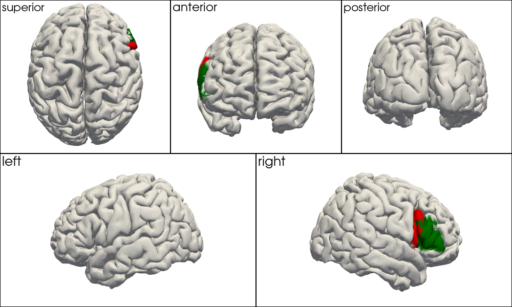
Pattern 2 — highlight a set of parcels in a single color:

Pass a single color string as color_mapping and provide a labels list. Every vertex whose coordinate matches a label in the list gets the specified color; all other vertices get default_color. This gives the clearest signal-vs-background contrast when you want to show, for example, bilateral Broca’s area (BA44 + BA45) against a neutral grey background.

# specify only a single color, that will be used for all parcels. Then select only a subset of parcels to color.

vertex_colors = get_vertex_colors_from_coord(
    colin_ijk_labeled.brain,
    "parcel_brodmann",
    color_mapping="r",
    labels=["right_BA44", "right_BA45"],
)
plot_brain_views_grid(colin_ijk_labeled.brain, vertex_colors)

Spot-Check: Verifying Label Assignments at Known MNI Coordinates

As a sanity check we verify that the assigned labels are anatomically plausible at three well-known MNI152 locations. We find the nearest brain surface vertex in MNI152 space and read off its Brodmann label.

MNI coordinate	Expected region
[-10, -90, 0]	Occipital pole / calcarine sulcus (BA17/18)
[-40, -20, 50]	Left somatomotor cortex (BA4/6)
[ 40,  20, 30]	Right prefrontal cortex (BA44/45/46)

tests = np.asarray([
    [-10, -90, 0],
    [-40, -20, 50],
    [40, 20, 30],
], dtype=float)

vertex_coords = icbm_ijk_labeled.get_brain_mni152_coords().pint.dequantify().values
vertex_labels = icbm_ijk_labeled.brain.vertices.coords["parcel_brodmann"].values
_, nearest = KDTree(vertex_coords).query(tests)

for mni, vertex_idx in zip(tests, nearest):
    print(f"MNI {mni.tolist()} -> nearest surface label {vertex_labels[vertex_idx]}")

MNI [-10.0, -90.0, 0.0] -> nearest surface label left_BA17
MNI [-40.0, -20.0, 50.0] -> nearest surface label left_BA3
MNI [40.0, 20.0, 30.0] -> nearest surface label right_BA44

Parcel-Level Summary Tables

TwoSurfaceHeadModel.parcel_summary_from_vertex_coordinate converts the per-vertex atlas labels into a compact table with one row per Schaefer2018 parcel (the parcellation bundled with the head model). For each Schaefer parcel it reports:

Column	Meaning
atlas_label	Dominant atlas region covering that parcel (plurality vote over vertices)
matching_vertices	Number of vertices whose atlas label equals atlas_label
parcel_vertices	Total number of vertices in the Schaefer parcel
fraction_of_parcel	Coverage fraction (matching_vertices / parcel_vertices)
mni152_r/a/s	MNI152 centroid of a representative vertex from that parcel

Medial-wall and background parcels are excluded by default because they do not correspond to cortical tissue. The function returns a pandas.DataFrame that can be saved with .to_csv(..., sep='\t') for use in downstream analyses or supplementary tables in manuscripts.

colin_ijk_labeled.parcel_summary_from_vertex_coordinate("parcel_aal3", "colin27")

	model	parcel	atlas_label	vertex	fsaverage_vertex	mni152_r	mni152_a	mni152_s	matching_vertices	parcel_vertices	fraction_of_parcel
0	colin27	ContA_Cingm_1_LH	Cingulate_Mid_L	6050	81691	-4.194	-10.030	33.413	12	12	1.000000
1	colin27	ContA_Cingm_1_RH	Cingulate_Mid_R	18544	249911	5.843	-8.805	33.371	11	13	0.846154
2	colin27	ContA_IPS_1_LH	Parietal_Sup_L	1219	15719	-28.909	-75.494	47.774	10	20	0.500000
3	colin27	ContA_IPS_1_RH	Angular_R	13549	181020	36.346	-73.024	43.556	18	25	0.720000
4	colin27	ContA_IPS_2_LH	Parietal_Inf_L	4075	51449	-59.949	-37.912	41.309	23	29	0.793103
...	...	...	...	...	...	...	...	...	...	...	...
595	colin27	VisPeri_StriCal_3_LH	Calcarine_L	223	3101	-1.603	-93.161	10.735	36	50	0.720000
596	colin27	VisPeri_StriCal_3_RH	Calcarine_R	13024	174186	14.307	-82.023	13.997	110	110	1.000000
597	colin27	VisPeri_StriCal_4_LH	Calcarine_L	589	8138	-6.291	-84.121	13.808	85	87	0.977011
598	colin27	VisPeri_StriCal_4_RH	Calcarine_R	13720	183134	26.726	-69.642	7.819	64	71	0.901408
599	colin27	VisPeri_StriCal_5_LH	Calcarine_L	381	5258	-0.509	-89.682	6.975	21	52	0.403846

600 rows × 11 columns

colin_ijk_labeled.parcel_summary_from_vertex_coordinate("parcel_brodmann", "colin27")

	model	parcel	atlas_label	vertex	fsaverage_vertex	mni152_r	mni152_a	mni152_s	matching_vertices	parcel_vertices	fraction_of_parcel
0	colin27	ContA_Cingm_1_LH	left_BA24	6118	82796	-2.442	-8.436	33.461	9	12	0.750000
1	colin27	ContA_Cingm_1_RH	right_BA24	18758	253120	3.221	-5.799	32.801	9	13	0.692308
2	colin27	ContA_IPS_1_LH	left_BA39	1219	15719	-28.909	-75.494	47.774	11	20	0.550000
3	colin27	ContA_IPS_1_RH	right_BA39	13549	181020	36.346	-73.024	43.556	23	25	0.920000
4	colin27	ContA_IPS_2_LH	left_BA40	4075	51449	-59.949	-37.912	41.309	25	29	0.862069
...	...	...	...	...	...	...	...	...	...	...	...
595	colin27	VisPeri_StriCal_3_LH	left_BA17	344	4710	-5.828	-90.400	10.766	28	50	0.560000
596	colin27	VisPeri_StriCal_3_RH	right_BA17	13024	174186	14.307	-82.023	13.997	109	110	0.990909
597	colin27	VisPeri_StriCal_4_LH	left_BA17	591	8168	-7.531	-83.706	11.621	76	87	0.873563
598	colin27	VisPeri_StriCal_4_RH	right_BA17	13720	183134	26.726	-69.642	7.819	59	71	0.830986
599	colin27	VisPeri_StriCal_5_LH	right_BA17	683	9407	1.304	-82.129	8.227	17	52	0.326923

600 rows × 11 columns

icbm_ijk_labeled.parcel_summary_from_vertex_coordinate("parcel_aal3", "icbm152")

	model	parcel	atlas_label	vertex	fsaverage_vertex	mni152_r	mni152_a	mni152_s	matching_vertices	parcel_vertices	fraction_of_parcel
0	icbm152	ContA_Cingm_1_LH	Cingulate_Mid_L	6306	85636	-3.545	-2.610	31.203	8	12	0.666667
1	icbm152	ContA_Cingm_1_RH	Cingulate_Mid_R	18374	240857	3.967	-8.118	30.450	18	21	0.857143
2	icbm152	ContA_IPS_1_LH	Occipital_Mid_L	783	10677	-30.465	-78.741	40.341	14	20	0.700000
3	icbm152	ContA_IPS_1_RH	Occipital_Mid_R	13573	174981	29.782	-73.129	31.792	10	14	0.714286
4	icbm152	ContA_IPS_2_LH	Parietal_Inf_L	2895	38740	-59.714	-50.221	46.333	45	48	0.937500
...	...	...	...	...	...	...	...	...	...	...	...
595	icbm152	VisPeri_StriCal_3_LH	Calcarine_L	202	2951	-6.776	-90.375	6.044	31	41	0.756098
596	icbm152	VisPeri_StriCal_3_RH	Calcarine_R	12837	164441	8.545	-87.583	7.512	89	102	0.872549
597	icbm152	VisPeri_StriCal_4_LH	Calcarine_L	554	7518	-11.499	-81.603	7.934	67	71	0.943662
598	icbm152	VisPeri_StriCal_4_RH	Calcarine_R	13479	173545	23.424	-74.785	7.149	43	56	0.767857
599	icbm152	VisPeri_StriCal_5_LH	Calcarine_L	383	5319	-7.192	-86.332	5.366	32	37	0.864865

600 rows × 11 columns

icbm_ijk_labeled.parcel_summary_from_vertex_coordinate("parcel_brodmann", "icbm152")

	model	parcel	atlas_label	vertex	fsaverage_vertex	mni152_r	mni152_a	mni152_s	matching_vertices	parcel_vertices	fraction_of_parcel
0	icbm152	ContA_Cingm_1_LH	left_BA24	5919	80515	-0.747	-7.566	32.542	11	12	0.916667
1	icbm152	ContA_Cingm_1_RH	right_BA24	18374	240857	3.967	-8.118	30.450	20	21	0.952381
2	icbm152	ContA_IPS_1_LH	left_BA39	783	10677	-30.465	-78.741	40.341	18	20	0.900000
3	icbm152	ContA_IPS_1_RH	right_BA7	13818	178245	26.570	-69.859	39.936	8	14	0.571429
4	icbm152	ContA_IPS_2_LH	left_BA40	2895	38740	-59.714	-50.221	46.333	48	48	1.000000
...	...	...	...	...	...	...	...	...	...	...	...
595	icbm152	VisPeri_StriCal_3_LH	left_BA17	202	2951	-6.776	-90.375	6.044	39	41	0.951220
596	icbm152	VisPeri_StriCal_3_RH	right_BA17	12837	164441	8.545	-87.583	7.512	92	102	0.901961
597	icbm152	VisPeri_StriCal_4_LH	left_BA17	554	7518	-11.499	-81.603	7.934	71	71	1.000000
598	icbm152	VisPeri_StriCal_4_RH	right_BA17	13479	173545	23.424	-74.785	7.149	49	56	0.875000
599	icbm152	VisPeri_StriCal_5_LH	left_BA17	383	5319	-7.192	-86.332	5.366	29	37	0.783784

600 rows × 11 columns

Optional: Save Summary Tables

The summary tables above are ordinary pandas.DataFrame objects. To write them to disk, set SAVE_TABLES = True in the next cell. Files are saved in the atlas_parcel_summaries/ folder relative to the notebook kernel’s current working directory.

from pathlib import Path

SAVE_TABLES = False
OUTPUT_DIR = Path("atlas_parcel_summaries")

if SAVE_TABLES:
    OUTPUT_DIR.mkdir(parents=True, exist_ok=True)
    summaries = {
        "aal3_parcel_summary_colin27.tsv": colin_ijk_labeled.parcel_summary_from_vertex_coordinate("parcel_aal3", "colin27"),
        "brodmann_parcel_summary_colin27.tsv": colin_ijk_labeled.parcel_summary_from_vertex_coordinate("parcel_brodmann", "colin27"),
        "aal3_parcel_summary_icbm152.tsv": icbm_ijk_labeled.parcel_summary_from_vertex_coordinate("parcel_aal3", "icbm152"),
        "brodmann_parcel_summary_icbm152.tsv": icbm_ijk_labeled.parcel_summary_from_vertex_coordinate("parcel_brodmann", "icbm152"),
    }
    for filename, summary in summaries.items():
        summary.to_csv(OUTPUT_DIR / filename, sep="\t", index=False)
    print(f"Saved {len(summaries)} summary tables to {OUTPUT_DIR.resolve()}")

Limitations of the Volumetric MNI Approach

Why parcel borders appear fuzzy on the inflated surface

The volumetric-to-surface label transfer is inherently approximate. The label of a brain surface vertex is determined by the nearest labelled voxel in 3-D MNI152 space. Because sulcal folds can bring two cortically distant regions to within a few millimetres of each other in 3-D, vertices near a sulcal wall may be assigned the label of the anatomically adjacent — but cortically distant — region instead of their own.

This artefact is most visible on the inflated surface: inflation changes vertex positions in 3-D while leaving labels fixed. Vertices that sit at the fundus (bottom) of a deep sulcus can therefore show “bleeding” — incorrect labels — at the inflated parcel border, even though the label assignment on the folded pial surface appears correct.

The mni_eps search radius controls the trade-off: a smaller radius reduces cross-sulcal contamination but increases the number of vertices that receive 'Background' (no labelled voxel found within reach). The default of 5 mm is a practical compromise for atlases with 1 mm isotropic voxels.

When to use FreeSurfer-based labeling instead

For applications where parcel boundary precision matters — for example when comparing fine-grained DOT image reconstruction results to specific cortical regions, or when building a classifier that relies on exact parcel membership — surface-native labeling via FreeSurfer is the more accurate alternative.

FreeSurfer [Fis12] assigns parcels directly on the cortical surface mesh by registering each vertex to the fsaverage template, where parcel boundaries are defined as vertex-level annotations. Because the boundary is expressed in the same surface space as the vertex, no voxel-lookup approximation is introduced and region borders are exact, even on the inflated surface.

Cedalion provides a complete FreeSurfer-based pipeline for individualized head models in 43b_individualized_head_models.ipynb, which walks through FreeSurfer cortical reconstruction, registration to fsaverage, and surface-native parcel annotation. The standard Colin27 and ICBM152 models were built with exactly this pipeline; their bundled parcel coordinate (Schaefer2018) is a surface-native annotation — which is why Schaefer borders look sharper than AAL3 or Brodmann borders on the same inflated surface.

Practical guidance:

Use case	Recommended approach
Quick atlas comparison, ROI definitions, group-level reporting	Volumetric MNI lookup (this notebook)
High-precision boundary analysis, individual MRI available	FreeSurfer surface-native labeling
Bridging a new atlas to an existing surface-native parcellation	Volumetric MNI lookup, compare overlap with Schaefer via parcel_summary_from_vertex_coordinate

References

cedalion.bib.dump_to_notebook()

Methods used

[1]	Holmes1998	cedalion.data.get_colin27_headmodel_files	Colin J. Holmes, Rick Hoge, Louis Collins, Roger Woods, Arthur W. Toga, and Alan C. Evans. Enhancement of mr images using registration for signal averaging. Journal of Computer Assisted Tomography, 22(2):324–333, March 1998. doi:10.1097/00004728-199803000-00032.
[2]	Fischl2012	cedalion.data.get_colin27_headmodel_files, cedalion.data.get_icbm152_headmodel_files	Bruce Fischl. FreeSurfer. NeuroImage, 62(2):774–781, 2012. doi:10.1016/j.neuroimage.2012.01.021.
[3]	Schaefer2018	cedalion.data.get_colin27_headmodel_files, cedalion.data.get_icbm152_headmodel_files	Alexander Schaefer, Ru Kong, Evan M Gordon, Timothy O Laumann, Xi-Nian Zuo, Avram J Holmes, Simon B Eickhoff, and BT Thomas Yeo. Local-global parcellation of the human cerebral cortex from intrinsic functional connectivity mri. Cerebral cortex, 28(9):3095–3114, 2018. doi:10.1093/cercor/bhx179.
[4]	Fonov2011	cedalion.data.get_icbm152_headmodel_files	Vladimir Fonov, Alan C. Evans, Kelly Botteron, C. Robert Almli, Robert C. McKinstry, and D. Louis Collins. Unbiased average age-appropriate atlases for pediatric studies. NeuroImage, 54(1):313–327, January 2011. doi:10.1016/j.neuroimage.2010.07.033.
[5]	Rolls2020	cedalion.data.get_atlas_files	Edmund T. Rolls, Chu-Chung Huang, Ching-Po Lin, Jianfeng Feng, and Marc Joliot. Automated anatomical labelling atlas 3. NeuroImage, 206:116189, 2020. doi:https://doi.org/10.1016/j.neuroimage.2019.116189.
[6]	Mai2017	cedalion.data.get_atlas_files	Jürgen K. Mai and Milan Majtanik. Human Brain in Standard MNI Space: Structure and Function: A Comprehensive Pocket Atlas. Academic Press, an imprint of Elsevier, London ; San Diego, CA, 2017. ISBN 978-0-12-811275-5.