S2: Photogrammetric Optode Co-Registration
Photogrammetry offers a possibility to get subject-specific optode coordinates. This notebook illustrates the individual steps to obtain these coordinates from a textured triangle mesh and a predefined montage.
Learning objectives
In this notebook you will learn to:
Understand what photogrammetry is and why it is used for fNIRS optode localisation
Use Cedalion’s photogrammetric registration to align a scalp scan to the head model
Visualise the co-registration result and assess alignment quality
[1]:
# This cells setups the environment when executed in Google Colab.
try:
    import google.colab
    !curl -s https://raw.githubusercontent.com/ibs-lab/cedalion/dev/scripts/colab_setup.py -o colab_setup.py
    # Select branch with --branch "branch name" (default is "dev")
    %run colab_setup.py
except ImportError:
    pass
[2]:
import matplotlib.image as mpimg
import matplotlib.pyplot as plt

import pyvista as pv
import xarray as xr

import cedalion
import cedalion.dataclasses as cdc
import cedalion.data
import cedalion.geometry.registration
import cedalion.io
import cedalion.vis
import cedalion.vis.blocks as vbx
from cedalion.vis.anatomy import OptodeSelector
from cedalion.geometry.photogrammetry.processors import (
    ColoredStickerProcessor,
    geo3d_from_scan,
)
from cedalion.geometry.registration import find_spread_points
from tempfile import TemporaryDirectory
from pathlib import Path


xr.set_options(display_expand_data=False)
[2]:
<xarray.core.options.set_options at 0x7f350d2b5050>
0. Choose between interactive and static mode
This example notebook provides two modes, controlled by the constant INTERACTIVE:
a static mode intended for rendering the documentation
an interactive mode, in which the 3D visualizations react to user input. The camera position can be changed. More importantly, the optode and landmark picking needs these interactive plots.
[3]:
INTERACTIVE = False

if INTERACTIVE:
    # option 1: render in the browser
    # pv.set_jupyter_backend("client")
    # option 2: offload rendering to a server process using trame
    pv.set_jupyter_backend("server")
else:
    pv.set_jupyter_backend("static")  # static rendering (for documentation page)
1. Loading the triangulated surface mesh
Use cedalion.io.read_einstar_obj to read the textured triangle mesh produced by the Einstar scanner. By default we use an example dataset. By setting the fname_ variables the notebook can operate on another scan.
[4]:
# insert here your own files if you do not want to use the example
fname_scan = ""  # path to .obj scan file
fname_snirf = "" # path to .snirf file for montage information
fname_montage_img = "" # path to an image file of the montage

if not fname_scan:
    fname_scan, fname_montage_img = (
        cedalion.data.get_fingertappingDOT_photogrammetry_scan()
    )

surface_mesh = cedalion.io.read_einstar_obj(fname_scan)
display(surface_mesh)
TrimeshSurface(faces: 1170428 vertices: 628185 crs: digitized units: millimeter vertex_coords: [])
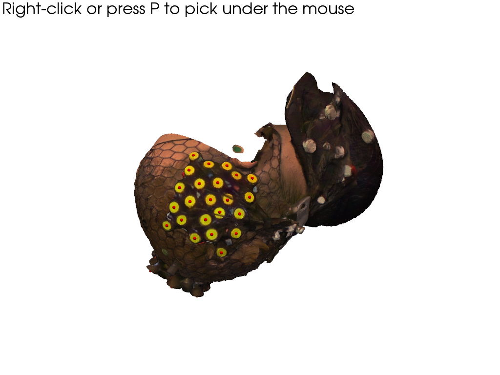
2. Identifying sticker vertices
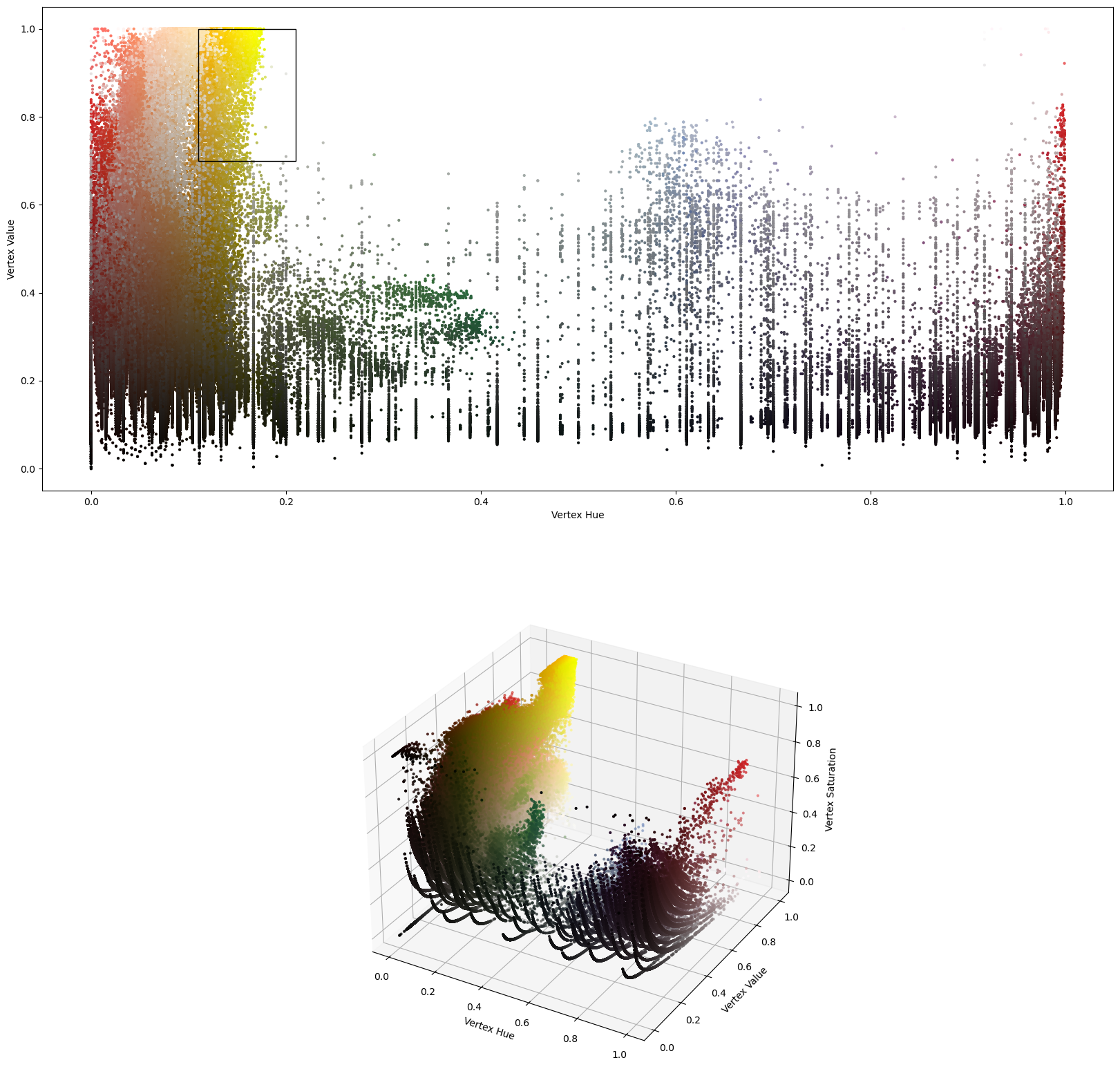
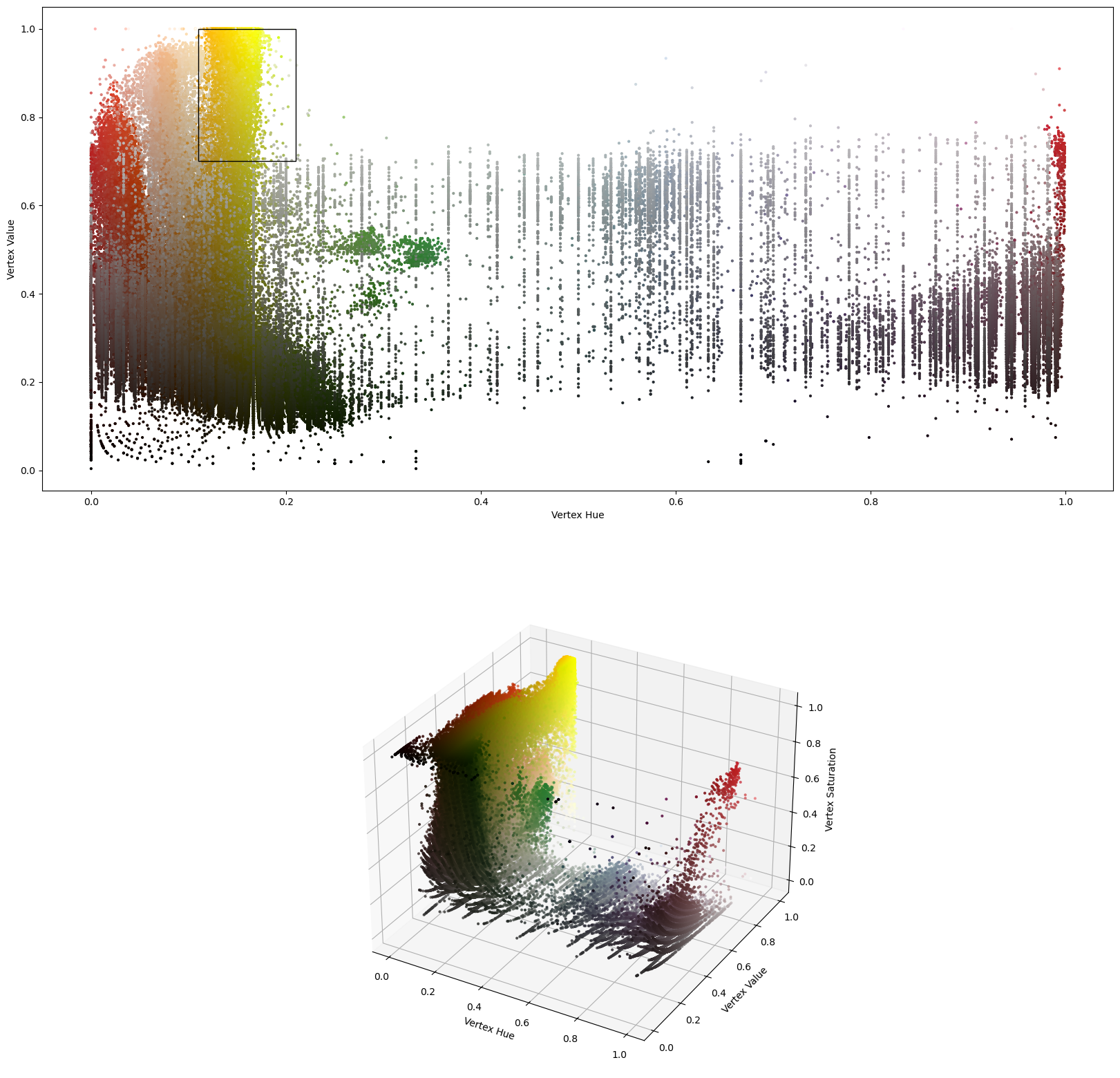
Processors are meant to analyze the textured mesh and extract positions. The ColoredStickerProcessor searches for colored vertices that form circular areas. We operate in HSV color space and the colors must be specified by their ranges in hue and value. These can be found by usig a color pipette tool on the texture file.
Multiple classes with different colors can be specified. In the following only yellow stickers for class “O(ptode)” are searched. But it could be extended to search also for differently colored sticker. (e.g. “L(andmark)”).
For each sticker the center and the normal is derived. Labels are generated from the class name and a counter, e.g. “O-01, O-02, …”
[5]:
processor = ColoredStickerProcessor(
    colors={
        "O" : ((0.11, 0.21, 0.7, 1)), # (hue_min, hue_max, value_min, value_max)
        #"L" : ((0.25, 0.37, 0.35, 0.6))
    }
)

# Select the hue and value ranges based on this preview of the distribution of
# vertices in color space.
preview_details = processor.inspect_colors(surface_mesh)
preview_details.plot_vertex_colors()
[6]:
# process the mesh
sticker_centers, normals, details = processor.process(surface_mesh, details=True)
display(sticker_centers)
[[172.506348 168.70253  570.348572]
 [150.027954  86.302536 570.348572]
 [172.497742 169.502548 570.348572]
 ...
 [146.47406  217.239182 493.978607]
 [145.855286 217.494583 493.578003]
 [145.55806  217.509079 493.342957]]
[[153.826904 253.747421 570.348572]
 [152.226929 254.987106 570.348572]
 [151.426941 255.54277  570.348572]
 ...
 [147.931213 179.410263 446.350281]
 [146.85408  180.071243 446.188019]
 [148.198898 179.035706 446.32309 ]]
O (0.11, 0.21, 0.7, 1)
[0.08044177 0.13082995 0.33646228 0.11412244 0.25736438 0.11922193
 0.4153435  0.03535901 0.07084033 0.05099133 0.02689893 0.01353992
 0.2012572  0.10884814 0.13261828 0.09033008 0.02105115 0.36269092
 0.46121203 0.18653857 0.08298083 0.08889661 0.1213103  0.32902637
 0.10617724 0.13214465 0.02324206 0.04296863 0.22714917 0.16556811
 0.07966138 0.51736194 0.22815784 0.04237109 0.3412102  1.30951184
 0.10917468 0.00800159 0.58517163 0.23383349 0.26694934 2.72721173
 0.0205321  0.67452466 0.4052373  0.312755   0.27754834]
5.791657838212683
surface.crs digitized
<xarray.DataArray (label: 47, digitized: 3)> Size: 1kB
[mm] 171.3 195.1 608.5 146.5 152.2 448.6 ... 123.8 236.1 615.8 142.3 240.5 603.4
Coordinates:
  * label    (label) <U4 752B 'O-38' 'O-12' 'O-43' ... 'O-44' 'O-36' 'O-42'
    type     (label) object 376B PointType.UNKNOWN ... PointType.UNKNOWN
    group    (label) <U1 188B 'O' 'O' 'O' 'O' 'O' 'O' ... 'O' 'O' 'O' 'O' 'O'
Dimensions without coordinates: digitizedVisualize the surface and extraced results.
[7]:
pvplt = pv.Plotter()
vbx.plot_surface(pvplt, surface_mesh, opacity=1.0)
vbx.plot_labeled_points(pvplt, sticker_centers, color="r")
vbx.plot_vector_field(pvplt, sticker_centers, normals)
vbx.camera_at_cog(pvplt, surface_mesh, (300,300,700),up=(1,0,0))
pvplt.show()
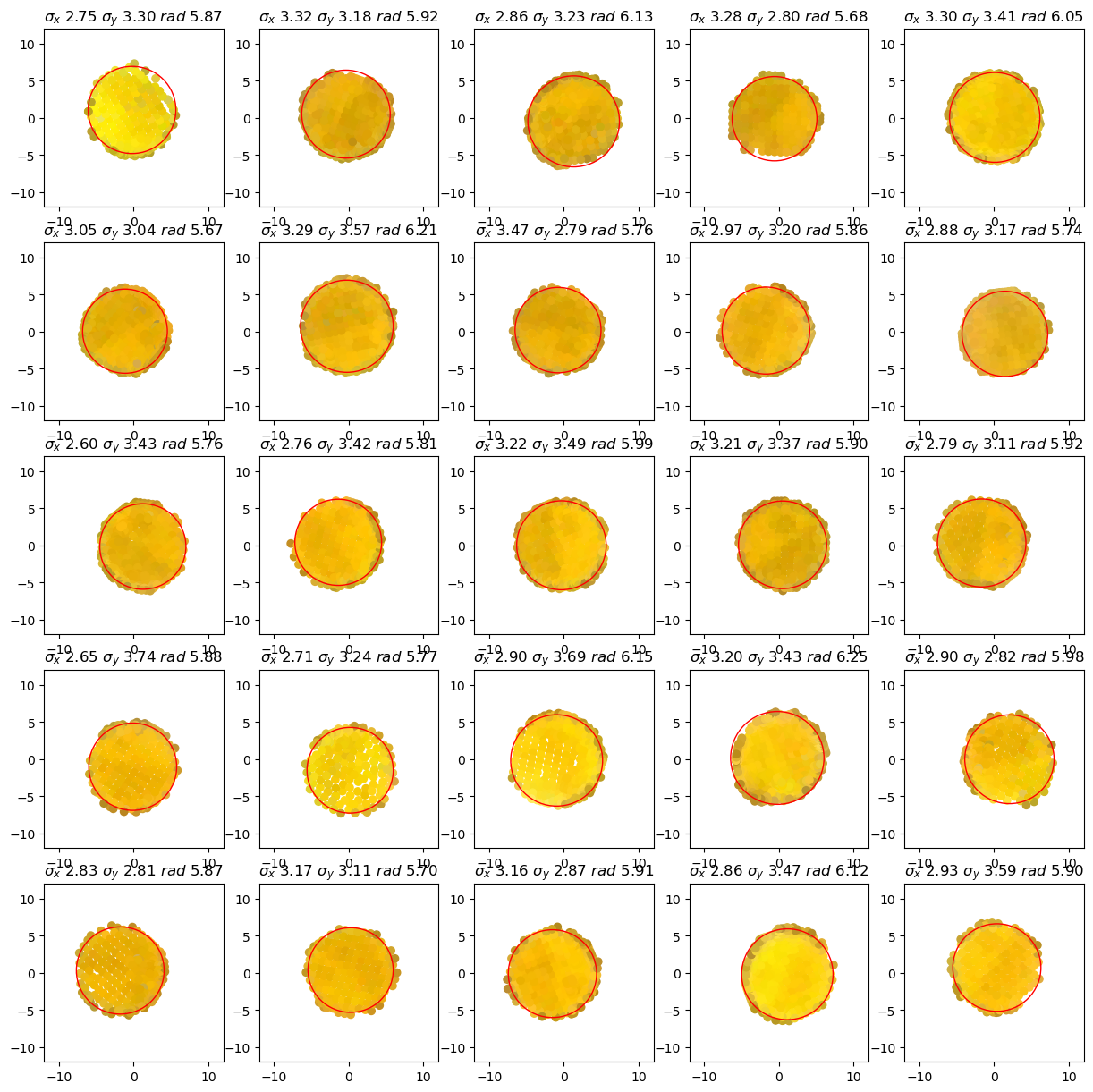
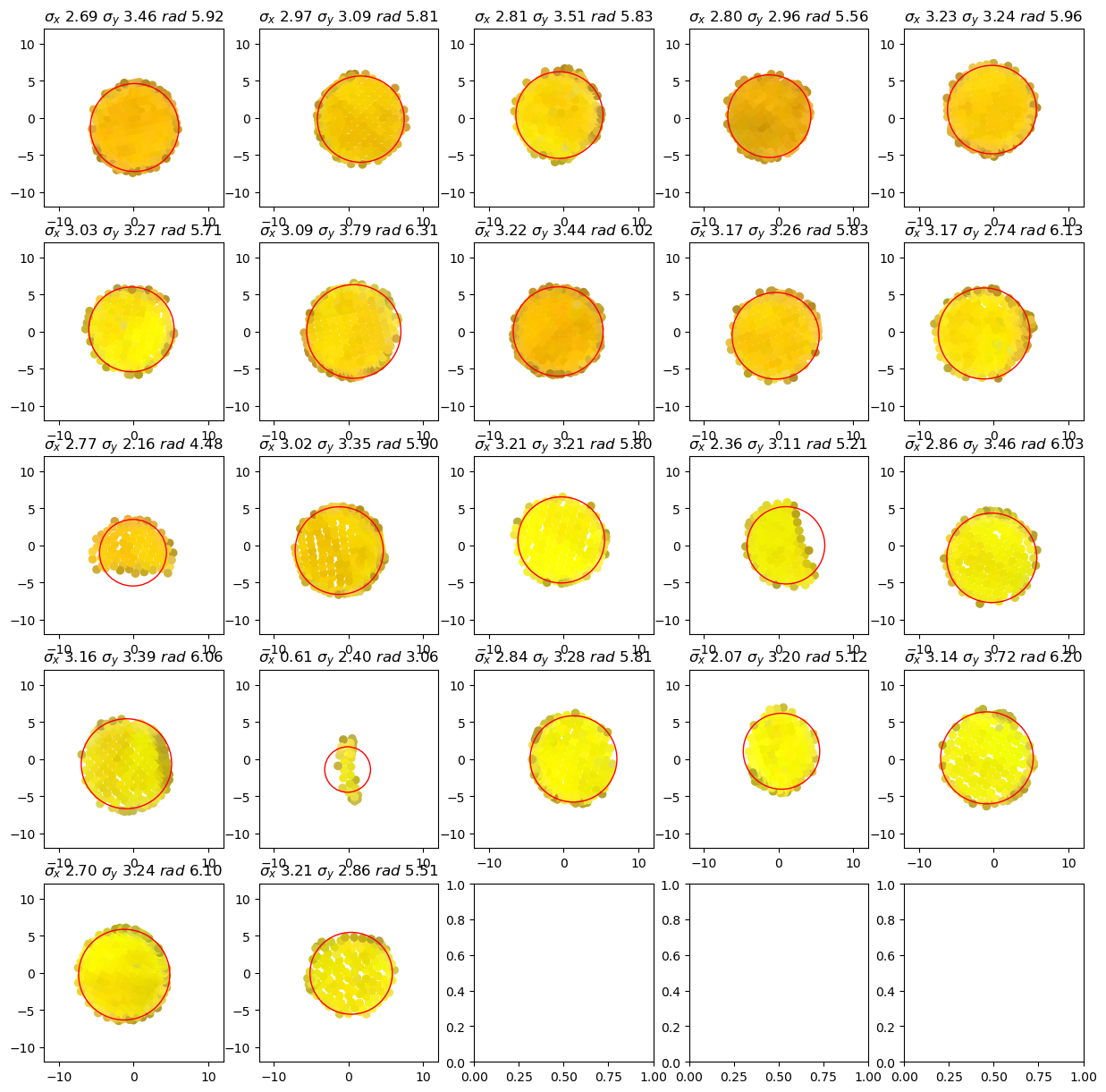
The details object is a container for debugging information and provides plotting functionality.
The following plots show for each cluster (tentative group of sticker vertices) The vertex positions perpendicular to the sticker normal as well as the minimum enclosing circle which is used to find the sticker’s center.
[8]:
details.plot_cluster_circles()
3. Manual corrections of sticker detection
If some optodes were misclassified or not all optodes were found automatically, there’s way to remove or add them manually.
In this example, a cable crosses the sticker of optode “D28” on the right hemisphere. The ColoredStickerProcessor misclassified the single sticker as two.
The OptodeSelect class provides an interactive visualization of the head scan and the detected stickers (red spheres):
By clicking with the right mouse button on:
a sphere, a misidentified sticker can be removed.
somewhere on the surface, a new sticker position can be added.
Use this, to remove the erroneously placed red sphere.
[9]:
optode_selector = OptodeSelector(surface_mesh, sticker_centers, normals)
optode_selector.plot()
optode_selector.enable_picking()
vbx.plot_surface(optode_selector.plotter, surface_mesh, opacity=1.0)

optode_selector.plotter.show()

Interactions modify the optode_selector.points and optode_selector.normals. After selecting all optodes, update sticker_centers and normals:
[10]:
sticker_centers = optode_selector.points.copy()
normals = optode_selector.normals.copy()

if not INTERACTIVE:
    sticker_centers = sticker_centers.drop_sel(label="O-42")
    normals = normals.drop_sel(label="O-42")

display(sticker_centers)
<xarray.DataArray (label: 46, digitized: 3)> Size: 1kB
[mm] 171.3 195.1 608.5 146.5 152.2 448.6 ... 184.3 195.8 589.3 123.8 236.1 615.8
Coordinates:
  * label    (label) <U4 736B 'O-38' 'O-12' 'O-43' ... 'O-39' 'O-44' 'O-36'
    type     (label) object 368B PointType.UNKNOWN ... PointType.UNKNOWN
    group    (label) <U1 184B 'O' 'O' 'O' 'O' 'O' 'O' ... 'O' 'O' 'O' 'O' 'O'
Dimensions without coordinates: digitized4. Project from sticker to scalp surface
Finally, to get from the sticker centers to the scalp coordinates we have to subtract the known lenght of the optodes in the direction of the normals:
[11]:
optode_length = 22.6 * cedalion.units.mm

scalp_coords = sticker_centers.copy()
mask_optodes = sticker_centers.group == "O"
scalp_coords[mask_optodes] = (
    sticker_centers[mask_optodes] - optode_length * normals[mask_optodes]
)
# we make a copy of this raw set of scalp coordinates to use later in the 2nd case of
# the coregistration example that showcases an alternative route if landmark-based
# coregistration fails
scalp_coords_altcase = scalp_coords.copy()

display(scalp_coords)
<xarray.DataArray (label: 46, digitized: 3)> Size: 1kB
[mm] 155.1 187.1 595.0 136.7 153.6 468.9 ... 165.2 189.2 579.2 117.1 222.3 599.2
Coordinates:
  * label    (label) <U4 736B 'O-38' 'O-12' 'O-43' ... 'O-39' 'O-44' 'O-36'
    type     (label) object 368B PointType.UNKNOWN ... PointType.UNKNOWN
    group    (label) <U1 184B 'O' 'O' 'O' 'O' 'O' 'O' ... 'O' 'O' 'O' 'O' 'O'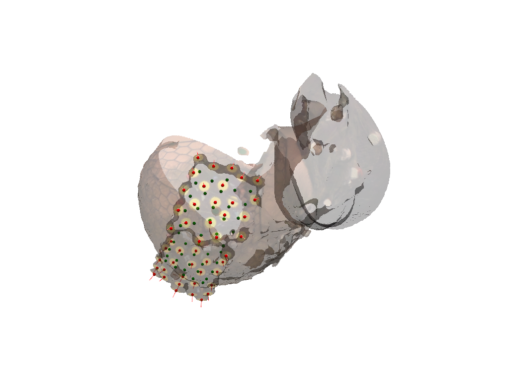
Dimensions without coordinates: digitizedVisualize sticker centers (red) and scalp coordinates (green).
[12]:
pvplt = pv.Plotter()
vbx.plot_surface(pvplt, surface_mesh, opacity=0.3)
vbx.plot_labeled_points(pvplt, sticker_centers, color="r")
vbx.plot_labeled_points(pvplt, scalp_coords, color="g")
vbx.plot_vector_field(pvplt, sticker_centers, normals)
pvplt.show()
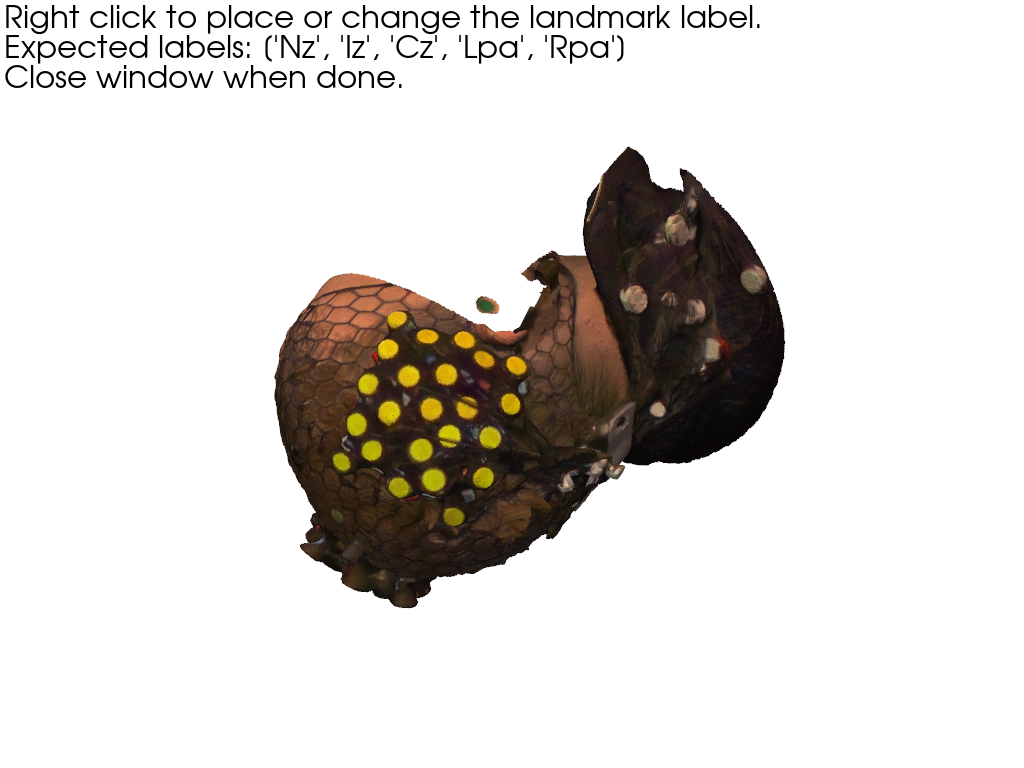
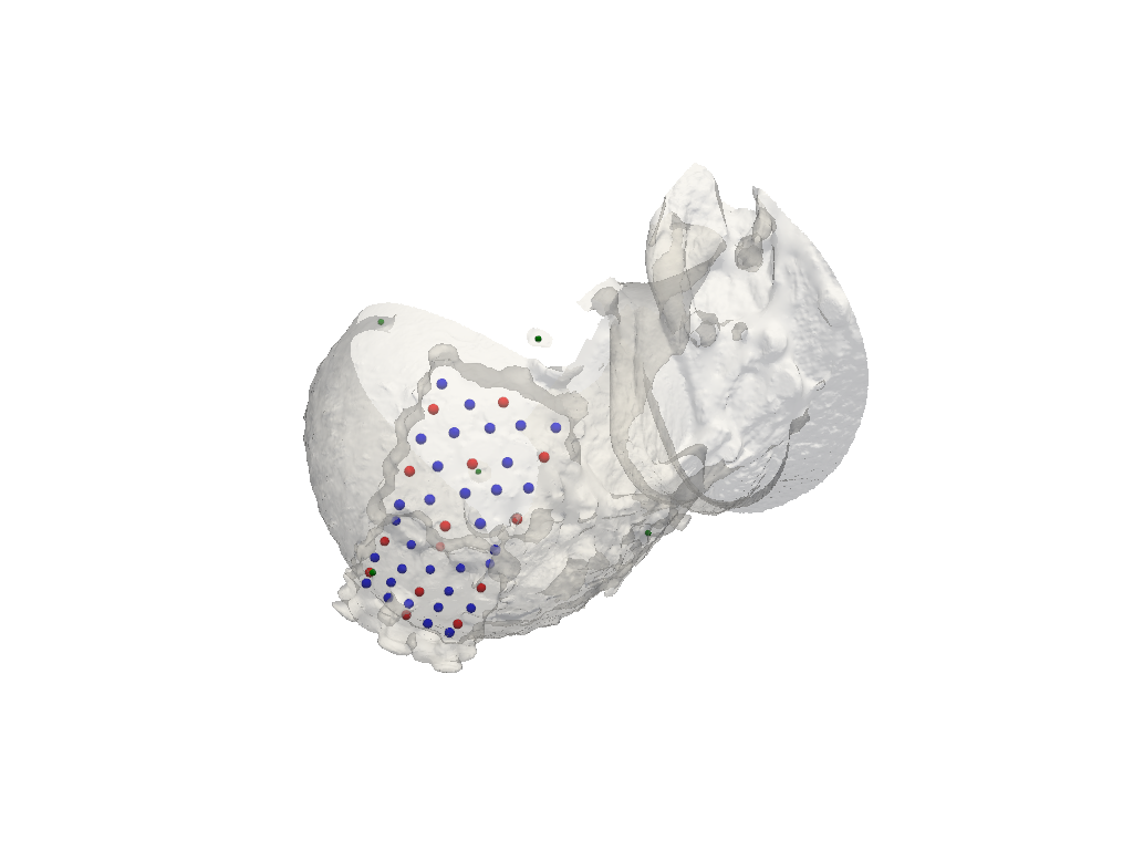
5. Specify landmarks on scanned head surface
5.1. Pick positions in interactive plot
When using the plot_surface function with parameter pick_landmarks set to True, the plot becomes interactive and allows to pick the positions of 5 landmarks. These are “Nz”, “Iz”, “Cz”, “Lpa”, “RpA”.
After clicking on the mesh, a green sphere marks the picked location. The sphere has a label attached. If this label is not visible, try to zoom further into the plot (mouse wheel). By clicking again with right mouse button on the sphere one can cycle through the different labels or remove a misplaced landmark.
It helps to add colored markers at the landmark positions when preparing the subject. Here green (Nz, Iz, Lpa, Rpa) and yellow (Cz) stickers where used. If the face is cropped from the scanned mesh for anonymization, make sure to preserve these stickers.
[13]:
pvplt = pv.Plotter()
get_landmarks = vbx.plot_surface(pvplt, surface_mesh, opacity=1.0, pick_landmarks=True)
pvplt.show()
5.2. Retrieve picked positions from interactive plot
The plot_surface function returns a function get_landmarks. Call this function to obtain:
1st value - coordinates of picked landmarks
2nd - labels of corresponding landmarks
[14]:
if INTERACTIVE:
    landmarks = get_landmarks()
else:
    # For documentation purposes and to enable automatically rendered example notebooks
    # we provide the hand-picked coordinates here, too.
    landmarks = xr.DataArray(
        [
            [ 68.64,  58.49, 594.20],
            [ 33.50, 249.85, 518.98],
            [176.69, 175.61, 530.85],
            [ 37.48, 107.10, 489.61],
            [ 48.39, 175.45, 624.98],
        ],
        dims=["label", "digitized"],
        coords={
            "label": ("label", ["Nz", "Iz", "Cz", "Lpa", "Rpa"]),
            "type": ("label", [cdc.PointType.LANDMARK] * 5),
            "group": ("label", ["L"] * 5),
        },
    ).pint.quantify("mm")

display(landmarks)

assert len(set(landmarks.label.values)) == 5, "please select 5 landmarks"
<xarray.DataArray (label: 5, digitized: 3)> Size: 120B
[mm] 68.64 58.49 594.2 33.5 249.8 519.0 ... 37.48 107.1 489.6 48.39 175.4 625.0
Coordinates:
  * label    (label) <U3 60B 'Nz' 'Iz' 'Cz' 'Lpa' 'Rpa'
    type     (label) object 40B PointType.LANDMARK ... PointType.LANDMARK
    group    (label) <U1 20B 'L' 'L' 'L' 'L' 'L'
Dimensions without coordinates: digitized6. Mapping the scanned optode positions to a predefined montage.
So far the optode positions found in the photogrammetric head scan carry only generic labels. In oder to identify them, they must be matched with a definition of the actual montage.
Snirf files store next to the actual time series data also the probe geometry, i.e. 3D coordinates of each source and detector. To label the optodes found in the photogrammetric scan, we map each optode to its counterpart in the snirf file.
The snirf coordinates are written during the data acquisition and are typically obtained by arranging the montage on a template head like ICBM-152 or colin27. So despite their similarity, the probe geometries in the snirf file and those from the head scan have differences because of different head geometries and different coordinate systems.
6.1 Load the montage information from .snirf file
[15]:
# read the example snirf file. Specify a name for the coordinate reference system.
if not fname_snirf:
    rec = cedalion.data.get_fingertappingDOT(crs="montage")
else:
    rec = cedalion.io.read_snirf(fname_snirf, crs="montage")[0]

# read 3D coordinates of the optodes
montage_elements = rec.geo3d

# landmark labels must match exactly. Adjust case where they don't match.
montage_elements = montage_elements.points.rename({"LPA": "Lpa", "RPA": "Rpa"})
6.2 Find a transformation to align selected landmarks to montage coordinates
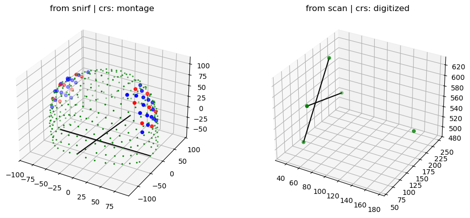
The coordinates in the snirf file and from the photogrammetric scan use different coordinate reference systems (CRS). In Cedalion the user needs to explicitly name different CRSs. Here the labels ‘digitized’ and ‘montage’ were used.
The following plot shows the probe geometry from the snirf file and the landmarks from the head scan. Two black lines Nz-Iz and Lpa-Rpa are added to guide the eye.
[16]:
f = plt.figure(figsize=(12,5))
ax1 = f.add_subplot(1,2,1, projection="3d")
ax2 = f.add_subplot(1,2,2, projection="3d")
colors = {cdc.PointType.SOURCE: "r", cdc.PointType.DETECTOR: "b"}
sizes = {cdc.PointType.SOURCE: 20, cdc.PointType.DETECTOR: 20}

for i, (type, x) in enumerate(montage_elements.groupby("type")):
    x = x.pint.to("mm").pint.dequantify()
    ax1.scatter(x[:, 0], x[:, 1], x[:, 2], c=colors.get(type, "g"), s=sizes.get(type, 2))

for i, (type, x) in enumerate(landmarks.groupby("type")):
    x = x.pint.to("mm").pint.dequantify()
    ax2.scatter(x[:, 0], x[:, 1], x[:, 2], c=colors.get(type, "g"), s=20)

for ax, points in [(ax1, montage_elements), (ax2, landmarks)]:
    points = points.pint.to("mm").pint.dequantify()
    ax.plot([points.loc["Nz",0], points.loc["Iz",0]],
            [points.loc["Nz",1], points.loc["Iz",1]],
            [points.loc["Nz",2], points.loc["Iz",2]],
            c="k"
            )
    ax.plot([points.loc["Lpa",0], points.loc["Rpa",0]],
            [points.loc["Lpa",1], points.loc["Rpa",1]],
            [points.loc["Lpa",2], points.loc["Rpa",2]],
            c="k"
            )

ax1.set_title(f"from snirf | crs: {montage_elements.points.crs}")
ax2.set_title(f"from scan | crs: {landmarks.points.crs}");
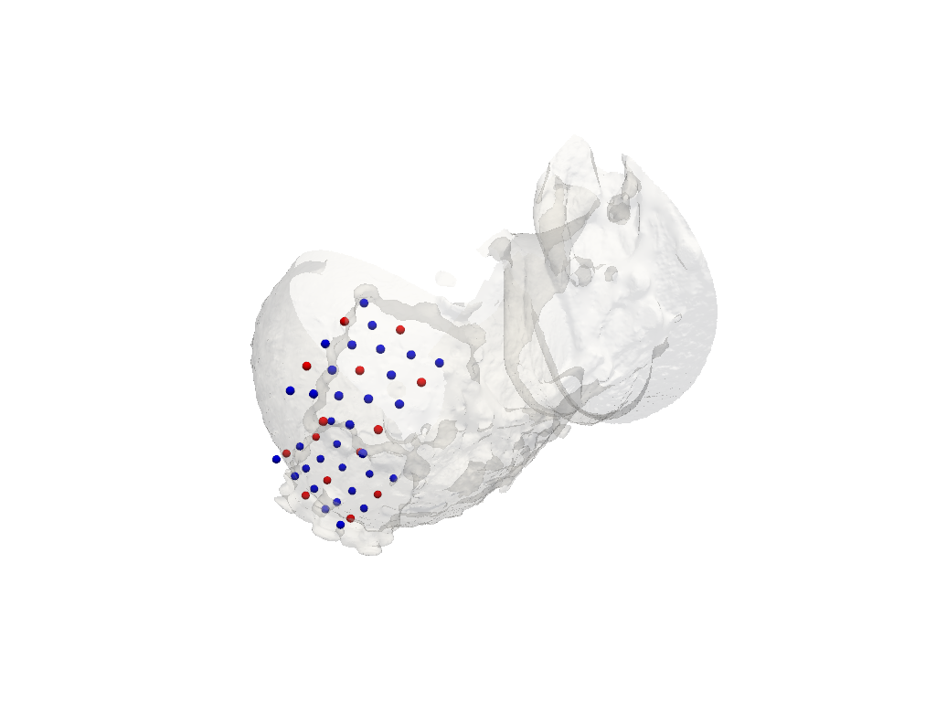
Subsequently, to bring the coordinates into the same space, from the landmarks a transformation (translations and rotations) is derived. This transforms the coordinates from the snirf file to the CRS of the photogramettric scan.
The following plot illustrates the transformed coordinates of sources (red) and detectors (blue). Deviations between these coordinates and the head surface are expected, since the optode positions where specified on a different head geometry.
[17]:
trafo = cedalion.geometry.registration.register_trans_rot(landmarks, montage_elements)

filtered_montage_elements = montage_elements.where(
    (montage_elements.type == cdc.PointType.SOURCE)
    | (montage_elements.type == cdc.PointType.DETECTOR),
    drop=True,
)
filtered_montage_elements_t = filtered_montage_elements.points.apply_transform(trafo)

pvplt = pv.Plotter()
vbx.plot_surface(pvplt, surface_mesh, color="w", opacity=.2)
vbx.plot_labeled_points(pvplt, filtered_montage_elements_t)
pvplt.show()
6.3 Iterative closest point algorithm to find labels for detected optode centers
Finally, the mapping is derived by iteratively trying to find a transformation that yilds the best match between the snirf and the scanned coordinates.
The following plot visualizes the result:
Green points represent optode centers
Next to them there shall be labels assumed by ICP algorithm (show_labels = True)
[18]:
# iterative closest point registration
idx = cedalion.geometry.registration.icp_with_full_transform(
    scalp_coords, filtered_montage_elements_t, max_iterations=100
)

# extract labels for detected optodes
label_dict = {}
for i, label in enumerate(filtered_montage_elements.coords["label"].values):
    label_dict[i] = label
labels = [label_dict[index] for index in idx]

# write labels to scalp_coords
scalp_coords = scalp_coords.assign_coords(label=labels)

# add landmarks
geo3Dscan = geo3d_from_scan(scalp_coords, landmarks)

display(geo3Dscan)
<xarray.DataArray (label: 51, digitized: 3)> Size: 1kB
[mm] 155.1 187.1 595.0 136.7 153.6 468.9 ... 37.48 107.1 489.6 48.39 175.4 625.0
Coordinates:
    type     (label) object 408B PointType.SOURCE ... PointType.LANDMARK
    group    (label) <U1 204B 'O' 'O' 'O' 'O' 'O' 'O' ... 'L' 'L' 'L' 'L' 'L'
  * label    (label) <U3 612B 'S9' 'D9' 'D23' 'D6' ... 'Iz' 'Cz' 'Lpa' 'Rpa'
Dimensions without coordinates: digitized
Attributes:
units: mm[19]:
f,ax = plt.subplots(1,2, figsize=(12,6))
cedalion.vis.anatomy.scalp_plot(
    rec["amp"],
    montage_elements,
    cedalion.nirs.channel_distances(rec["amp"], montage_elements),
    ax=ax[0],
    optode_labels=True,
    cb_label="channel dist. / mm",
    cmap="plasma",
    vmin=25,
    vmax=42,
)
ax[0].set_title("montage from snirf file")
cedalion.vis.anatomy.scalp_plot(
    rec["amp"],
    geo3Dscan,
    cedalion.nirs.channel_distances(rec["amp"], geo3Dscan),
    ax=ax[1],
    optode_labels=True,
    cb_label="channel dist. / mm",
    cmap="plasma",
    vmin=25,
    vmax=42,
)
ax[1].set_title("montage from photogrammetric scan")
plt.tight_layout()
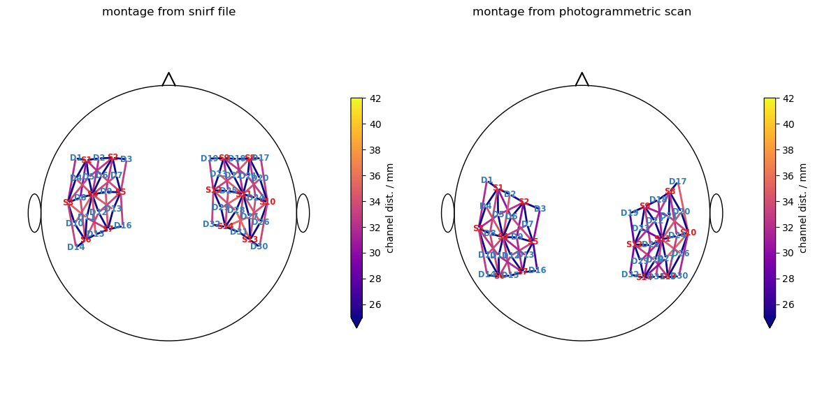
Visualization of successfull assignment (show_labels = True)
[20]:
pvplt = pv.Plotter()
cedalion.vis.anatomy.plot_brain_and_scalp(None, surface_mesh.mesh, None, None, plotter=pvplt)
vbx.plot_labeled_points(pvplt, geo3Dscan, show_labels=True)
pvplt.show()
6.4 Alternative approach without landmarks
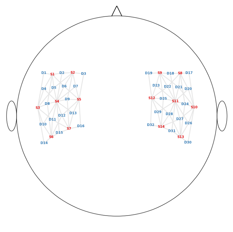
Mapping the optode labels can fail for example because of a bad landmark selection.
In such cases it is possible to find a new transformation by manually labeling three optodes. This is done by selecting them in a given order. For that it helps to have a visualization of the montage of your experiment.
[21]:
if fname_montage_img:
    # Load and display the image
    img = mpimg.imread(fname_montage_img)
    plt.figure(figsize=(12, 10))
    plt.imshow(img)
    plt.axis("off")  # Turn off axis labels and ticks
    plt.show()
else:
    print("No montage image specified.")
Search for three optodes that are evenly spreaded across the head surface. Afterwards prompt the user to right click on each of them.
[22]:
spread_point_labels = find_spread_points(filtered_montage_elements)
print("Select those points")
print(spread_point_labels)

points = []
pvplt = pv.Plotter()
vbx.plot_surface(pvplt, surface_mesh, opacity=1.0)
vbx.plot_labeled_points(pvplt, sticker_centers, color="r", ppoints = points)
pvplt.show()
/home/runner/miniconda3/envs/cedalion/lib/python3.11/site-packages/xarray/core/variable.py:315: UnitStrippedWarning: The unit of the quantity is stripped when downcasting to ndarray.
  data = np.asarray(data)
Select those points
['S1' 'D32' 'D10']
Retrieve picked positions:
[23]:
if INTERACTIVE:
    labeled_points = points
else:
    # For documentation purposes and to enable automatically rendered example notebooks
    # we provide the hand-picked coordinates here, too.
    labeled_points = [13, 12, 6]

display(labeled_points)

if len(labeled_points) != 3:
    raise ValueError("Please select the 3 specified points.")
[13, 12, 6]
Write the selected labels to the corresponding points of xarray.DataArray scalp_coords:
[24]:
new_labels = scalp_coords_altcase.label.values.copy()
for i, idx in enumerate(labeled_points):
    new_labels[idx] = spread_point_labels[i]
scalp_coords_altcase = scalp_coords_altcase.assign_coords(label=new_labels)
scalp_coords_altcase
[24]:
<xarray.DataArray (label: 46, digitized: 3)> Size: 1kB
[mm] 155.1 187.1 595.0 136.7 153.6 468.9 ... 165.2 189.2 579.2 117.1 222.3 599.2
Coordinates:
    type     (label) object 368B PointType.UNKNOWN ... PointType.UNKNOWN
    group    (label) <U1 184B 'O' 'O' 'O' 'O' 'O' 'O' ... 'O' 'O' 'O' 'O' 'O'
  * label    (label) <U4 736B 'O-38' 'O-12' 'O-43' ... 'O-39' 'O-44' 'O-36'
Dimensions without coordinates: digitizedFind the affine transformation for the newly labeled points and apply it to the montage optodes
[25]:
trafo2 = cedalion.geometry.registration.register_trans_rot(
    scalp_coords_altcase, montage_elements
)

filtered_montage_elements = montage_elements.where(
    (montage_elements.type == cdc.PointType.SOURCE)
    | (montage_elements.type == cdc.PointType.DETECTOR),
    drop=True,
)
filtered_montage_elements_t = filtered_montage_elements.points.apply_transform(trafo2)
and run ICP algorithm for label assignment once again, extract labels for detected optodes and plot the results
[26]:
# iterative closest point registration
idx = cedalion.geometry.registration.icp_with_full_transform(
    scalp_coords_altcase, filtered_montage_elements_t, max_iterations=100
)
# extract labels for detected optodes
label_dict = {}
for i, label in enumerate(filtered_montage_elements.coords["label"].values):
    label_dict[i] = label
labels = [label_dict[index] for index in idx]

# write labels to scalp_coords
scalp_coords_altcase = scalp_coords_altcase.assign_coords(label=labels)

# add landmarks
geo3Dscan_alt = geo3d_from_scan(scalp_coords_altcase, landmarks)
[27]:
f,ax = plt.subplots(1,2, figsize=(12,6))
cedalion.vis.anatomy.scalp_plot(
    rec["amp"],
    montage_elements,
    cedalion.nirs.channel_distances(rec["amp"], montage_elements),
    ax=ax[0],
    optode_labels=True,
    cb_label="channel dist. / mm",
    cmap="plasma",
    vmin=25,
    vmax=42,
)

ax[0].set_title("montage from snirf file")
cedalion.vis.anatomy.scalp_plot(
    rec["amp"],
    geo3Dscan_alt,
    cedalion.nirs.channel_distances(rec["amp"], geo3Dscan_alt),
    ax=ax[1],
    optode_labels=True,
    cb_label="channel dist. / mm",
    cmap="plasma",
    vmin=25,
    vmax=42,
)
ax[1].set_title("montage from photogrammetric scan")
plt.tight_layout()

7. Saving the result
Finally, the detected optode positions are stored to disk for later processing. Two approaches are shown: storing the coordinates in a BIDS-compliant TSV file, or storing them in a modified copy of the original SNIRF file.
Storing coordinates in a BIDS-compliant TSV file
[28]:
with TemporaryDirectory() as output_dir:
    # write result to temporary tsv file
    output_dir = Path(output_dir)
    tsv_filename = output_dir / "sub-01_optodes.tsv"

    cedalion.io.bids.export_to_bids_optodes_tsv(
        tsv_filename, geo3Dscan, float_format=".2f"
    )

    # reread written file and print first 10 lines
    with tsv_filename.open("r") as fin:
        print("".join(fin.readlines()[:10]))
name    type    x       y       z
S9      source  155.13  187.07  594.99
D9      detector        136.73  153.57  468.89
D23     detector        155.98  203.59  585.50
D6      detector        135.87  136.81  474.79
S2      source  148.13  133.26  487.91
D13     detector        138.09  172.12  465.88
D10     detector        88.19   145.23  462.33
S11     source  132.55  211.85  600.92
D21     detector        129.83  195.07  611.31
Storing coordinates in a SNIRF file
[29]:
with TemporaryDirectory() as output_dir:
    # take the original recording container and replace its geo3d attribute
    rec = cedalion.data.get_fingertappingDOT()
    rec.geo3d = geo3Dscan

    # write the result to a temporary snirf file
    output_dir = Path(output_dir)
    snirf_filename = output_dir / "snirf_with_scanned_optodes.snirf"
    cedalion.io.write_snirf(snirf_filename, rec)

    # reread the written file
    # SNIRF files do not label the coordinate reference system. Here, we specify the
    # name manually to match what we used before.
    loaded_rec = cedalion.io.read_snirf(snirf_filename, crs="digitized")[0]
    geo3d_loaded = loaded_rec.geo3d

    # the order of optodes in snirf's probe info. element may differ from geo3Dscan
    # assert that all optodes exist
    assert(sorted(geo3d_loaded.label.values) == sorted(geo3Dscan.label.values))

    # assert that all optode coordinates match geo3Dscan
    assert((geo3d_loaded.loc[geo3Dscan.label] == geo3Dscan).all())
References
[30]:
cedalion.bib.dump_to_notebook()
Methods used
| [1] | Tucker2022 | cedalion.io.snirf.read_snirf | Stephen Tucker, Jay Dubb, Sreekanth Kura, Alexander von Lühmann, Robert Franke, Jörn M. Horschig, Samuel Powell, Robert Oostenveld, Michael Lührs, Édouard Delaire, Zahra M. Aghajan, Hanseok Yun, Meryem A. Yücel, Qianqian Fang, Theodore J. Huppert, Blaise deB. Frederick, Luca Pollonini, David A. Boas, and Robert Luke. Introduction to the shared near infrared spectroscopy format. Neurophotonics, 10(1):013507, 2022. doi:10.1117/1.NPh.10.1.013507. |
| [2] | Gorgolewski2016 | cedalion.io.bids.export_to_bids_optodes_tsv | Krzysztof J. Gorgolewski, Tibor Auer, Vince D. Calhoun, R. Cameron Craddock, Samir Das, Eugene P. Duff, Guillaume Flandin, Satrajit S. Ghosh, Tristan Glatard, Yaroslav O. Halchenko, Daniel A. Handwerker, Michael Hanke, David Keator, Xiangrui Li, Zachary Michael, Camille Maumet, B. Nolan Nichols, Thomas E. Nichols, John Pellman, Jean-Baptiste Poline, Ariel Rokem, Gunnar Schaefer, Vanessa Sochat, William Triplett, Jessica A. Turner, Gaël Varoquaux, and Russell A. Poldrack. The brain imaging data structure, a format for organizing and describing outputs of neuroimaging experiments. Scientific Data, 3(1):160044, June 2016. doi:10.1038/sdata.2016.44. |
| [3] | Luke2025 | cedalion.io.bids.export_to_bids_optodes_tsv | Robert Luke, Robert Oostenveld, Helena Cockx, Guiomar Niso, Maureen J. Shader, Felipe Orihuela-Espina, Hamish Innes-Brown, Stephen Tucker, David Boas, Meryem A. Yücel, Remi Gau, Taylor Salo, Stefan Appelhoff, Christopher J. Markiewicz, David McAlpine, Luca Pollonini, and The BIDS Maintainers. NIRS-BIDS: Brain Imaging Data Structure Extended to Near-Infrared Spectroscopy. Scientific Data, 12(1):159, January 2025. doi:10.1038/s41597-024-04136-9. |
Next: 3 — Signal Processing — the full preprocessing pipeline.