Examining and thresholding sensitivity of a probe to the cortex using the Schaefer parcellation scheme
This notebook shows how to examine the theoretical sensitivity of a probe on a headmodel to brain areas (here we use parcel coordinates from the Schaefer 2018 atlas), and how to identify parcels that should be dropped, because changes in them cannot be observed. For this the original designed probe can also be reduced to an effective probe by dropping channels that are pruned due to bad signal quality.
[1]:
# This cells setups the environment when executed in Google Colab.
try:
    import google.colab
    !curl -s https://raw.githubusercontent.com/ibs-lab/cedalion/dev/scripts/colab_setup.py -o colab_setup.py
    # Select branch with --branch "branch name" (default is "dev")
    %run colab_setup.py
except ImportError:
    pass
[2]:
# set this flag to True to enable interactive 3D plots
INTERACTIVE_PLOTS = False
[3]:
import matplotlib.pyplot as p
import numpy as np
import pyvista as pv
import xarray as xr

import cedalion
import cedalion.data
import cedalion.dataclasses as cdc
import cedalion.dot as dot
import cedalion.sigproc.quality as quality
import cedalion.vis.anatomy.sensitivity_matrix
import cedalion.vis.blocks as vbx

if INTERACTIVE_PLOTS:
    pv.set_jupyter_backend('html')
else:
    pv.set_jupyter_backend('static')

xr.set_options(display_expand_data=False)

# for dev purposes
#%load_ext autoreload
#%autoreload 2
[3]:
<xarray.core.options.set_options at 0x7f432dc5f190>
Load a DOT finger-tapping dataset
and perform some very basic quality checks to identify bad channels
[4]:
# load example dataset
rec = cedalion.data.get_fingertappingDOT()

# check signal quality using a simple SNR threshold
snr_thresh = 30  # the SNR (std/mean) of a channel.
                 # Set very high here for demonstration purposes

# SNR thresholding using the "snr" function of the quality subpackage
snr, snr_mask = quality.snr(rec["amp"], snr_thresh)

# drop channels with bad signal quality (here we only need the list of channels):
# prune channels using the masks and the operator "all", which will keep only channels
# that pass all three metrics
_, snr_ch_droplist = quality.prune_ch(rec["amp"], [snr_mask], "all")

# print list of dropped channels
print(
    f"{len(snr_ch_droplist)} channels pruned. "
    f"List of pruned channels due to bad SNR: {snr_ch_droplist}"
)
37 channels pruned. List of pruned channels due to bad SNR: ['S1D1' 'S1D4' 'S1D5' 'S1D6' 'S1D8' 'S2D5' 'S2D6' 'S2D9' 'S3D1' 'S4D2'
 'S4D7' 'S4D13' 'S5D3' 'S5D6' 'S8D18' 'S8D20' 'S8D21' 'S8D22' 'S8D24'
 'S9D18' 'S9D21' 'S9D22' 'S9D25' 'S10D17' 'S10D21' 'S11D18' 'S11D20'
 'S11D23' 'S11D24' 'S11D29' 'S12D19' 'S12D22' 'S12D25' 'S12D28' 'S12D29'
 'S12D32' 'S14D27']
Load a headmodel and precalulated fluence profile
[5]:
head = dot.get_standard_headmodel("icbm152")

# snap probe to head and create forward model
geo3D_snapped = head.align_and_snap_to_scalp(rec.geo3d)

fwm = dot.ForwardModel(head, geo3D_snapped, rec._measurement_lists["amp"])
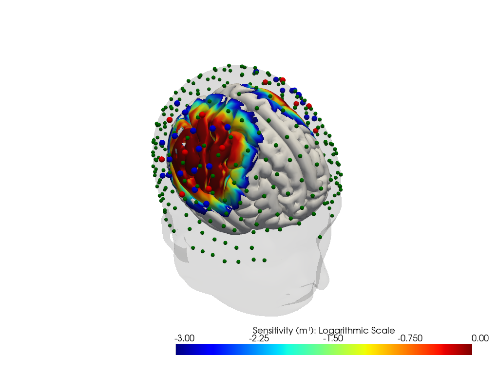
load precomputed fluce, calculate sensitivity on the cortex and plot it on head model
[6]:
# load precomputed sensitivity for this dataset and headmodel
Adot = cedalion.data.get_precomputed_sensitivity("fingertappingDOT", "icbm152")

# plot on head model
plotter = cedalion.vis.anatomy.sensitivity_matrix.Main(
    sensitivity=Adot,
    brain_surface=head.brain,
    head_surface=head.scalp,
    labeled_points=geo3D_snapped,
)
plotter.plot(high_th=0, low_th=-3)
plotter.plt.show()
Downloading file 'sensitivity_fingertappingDOT_icbm152.nc' from 'https://doc.ibs.tu-berlin.de/cedalion/datasets/dev/sensitivity_fingertappingDOT_icbm152.nc' to '/home/runner/.cache/cedalion/dev'.
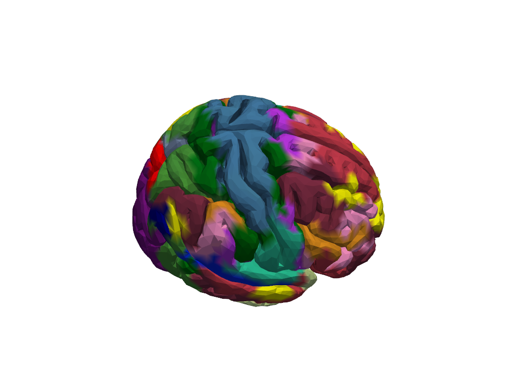
Investigation of Parcels and effective Parcel Sensitivity
First plot full parcellation scheme on head
[7]:
files = cedalion.data.get_icbm152_headmodel_files()
parcel_colors = cedalion.io.read_parcel_colors(files.basedir / files.parcel_colors)
[8]:
plt = pv.Plotter()
vbx.plot_surface(
    plt,
    head.brain,
    color=[
        parcel_colors.get(parcel, [0, 0, 0])
        for parcel in head.brain.vertices.parcel.values
    ],
    silhouette=True,
)
vbx.camera_at_cog(plt, head.brain, rpos=[400,0,400], fit_scene=True)
plt.show()
Calculate parcel sensitivity mask
Parcels are considered good, if a change in HbO and HbR [µMol] in the parcel leads to an observable change of at least dOD in at least one wavelength of one channel. Sensitivities of all vertices in the parcel are summed up in the sensitivity matrix Adot. Bad channels in an actual measurement that are pruned can be considered by providing a boolean channel_mask, where False indicates bad channels that are dropped and not considered for parcel sensitivity. Requires headmodel with parcelation coordinates.
For this the following input arguments are used with parcel_sensitivity():
Adot (channel, vertex, wavelength)): Sensitivity matrix with parcel coordinate belonging to each vertex
chan_mask: boolean xarray DataArray channel mask, False for channels to be dropped
dOD_thresh: threshold for minimum dOD change in a channel that should be observed from a hemodynamic change in a parcel
minCh: minimum number of channels per parcel that should see a change above dOD_thresh
dHbO: change in HbO concentration in the parcel in [µMol] used to calculate dOD
dHbR: change in HbR concentration in the parcel in [µMol] used to calculate dOD
Output is a tuple (parcel_dOD, parcel_mask), where
parcel_dOD (channel, parcel) contains the delta OD observed in a channel given the assumed dHb change in a parcel, and
parcel_mask is a boolean DataArray with parcel coords from Adot that is true for parcels for which dOD_thresh is met.
Example without channel pruning
[9]:
# set input parameters for parcel sensitivity calculation.
# Here we do not (yet) drop bad channels to investigate the genereal
# sensitivity of the probe to parcel space independent of channel quality

dOD_thresh = 0.001
minCh = 1
dHbO = 10  # µM
dHbR = -3  # µM

parcel_dOD, parcel_mask = fwm.parcel_sensitivity(
    Adot, None, dOD_thresh, minCh, dHbO, dHbR
)

# display results
display(parcel_dOD)
display(parcel_mask)

# fetch parcels from the parcel_mask that are above the threshold
# to a list of parcel names
sensitive_parcels = parcel_mask.where(parcel_mask, drop=True)["parcel"].values.tolist()
dropped_parcels = parcel_mask.where(~parcel_mask, drop=True)["parcel"].values.tolist()
print(f"Number of sensitive parcels: {len(sensitive_parcels)}")
print(f"Number of dropped parcels: {len(dropped_parcels)}")
<xarray.DataArray (wavelength: 2, channel: 100, parcel: 601)> Size: 962kB
1.285e-08 4.31e-13 6.683e-16 3.4e-18 ... 4.43e-13 1.58e-13 3.06e-13 5.396e-13
Coordinates:
  * channel     (channel) object 800B 'S1D1' 'S1D2' 'S1D4' ... 'S14D31' 'S14D32'
  * parcel      (parcel) object 5kB 'Background+FreeSurfer_Defined_Medial_Wal...
  * wavelength  (wavelength) float64 16B 760.0 850.0
<xarray.DataArray (parcel: 601)> Size: 601B
False False False False False True True ... False False False False False False
Coordinates:
  * parcel   (parcel) object 5kB 'Background+FreeSurfer_Defined_Medial_Wall' ...
Number of sensitive parcels: 107
Number of dropped parcels: 494
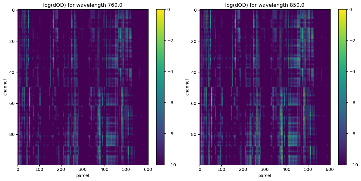
visualize results
[10]:
# plots a surface plot of dOD with axes "channel" and "parcel" using
# the log of the values in dOD on the z-axis for both wavelengths 760 and 850
fig, axes = p.subplots(1, 2, figsize=(12, 6))

for i, wl in enumerate([760.0, 850.0]):
    ax = axes[i]
    im = ax.imshow(np.log10(parcel_dOD.sel(wavelength=wl).values), aspect="auto")
    im.set_clim(-10, 0)
    fig.colorbar(im, ax=ax)
    ax.set_xlabel("parcel")
    ax.set_ylabel("channel")
    ax.set_title(f"log(dOD) for wavelength {wl}")

p.tight_layout()
p.show()
[11]:
# reduce parcel set to plot to the sensitive parcels
color = [
    parcel_colors[parcel] if parcel not in dropped_parcels else [1.0, 1.0, 1.0]
    for parcel in head.brain.vertices.parcel.values
]

plt = pv.Plotter()
vbx.plot_surface(plt, head.brain, color=color, silhouette=True)
vbx.camera_at_cog(plt, head.brain, [400,0,400], fit_scene=True)

# add probe
vbx.plot_labeled_points(
    plt, geo3D_snapped.sel(label=geo3D_snapped.label.str.contains("S|D"))
)
plt.show()

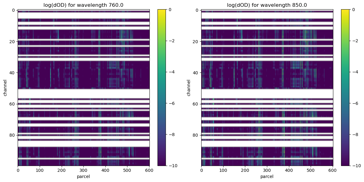
Example with channel pruning
The same as before, but now we consider a list of “bad” channels that should be excluded from the sensitivity consideration
[12]:
# set input parameters for parcel sensitivity calculation.
# Now we use the snr channel mask to exclude channels with bad signal quality
# (here artificially high threshold) from consideration for parcel sensitivity

dOD_thresh = 0.001
minCh = 1
dHbO = 10  # µMol
dHbR = -3  # µMol
chan_droplist = snr_ch_droplist  # list of dropped channels due to bad SNR,
                                 # effectively reducing probe


parcel_dOD, parcel_mask = fwm.parcel_sensitivity(
    Adot, chan_droplist, dOD_thresh, minCh, dHbO, dHbR
)

# display results
display(parcel_dOD)
display(parcel_mask)

# fetch parcels from the parcel_mask that are above the threshold
# to a list of parcel names
sensitive_parcels = parcel_mask.where(parcel_mask, drop=True)["parcel"].values.tolist()
dropped_parcels = parcel_mask.where(~parcel_mask, drop=True)["parcel"].values.tolist()
print(f"Number of sensitive parcels: {len(sensitive_parcels)}")
print(f"Number of dropped parcels: {len(dropped_parcels)}")
<xarray.DataArray (wavelength: 2, channel: 100, parcel: 601)> Size: 962kB
0.0 0.0 0.0 0.0 0.0 0.0 ... 9.404e-14 4.43e-13 1.58e-13 3.06e-13 5.396e-13
Coordinates:
  * channel     (channel) object 800B 'S1D1' 'S1D2' 'S1D4' ... 'S14D31' 'S14D32'
  * parcel      (parcel) object 5kB 'Background+FreeSurfer_Defined_Medial_Wal...
  * wavelength  (wavelength) float64 16B 760.0 850.0
<xarray.DataArray (parcel: 601)> Size: 601B
False False False False False True True ... False False False False False False
Coordinates:
  * parcel   (parcel) object 5kB 'Background+FreeSurfer_Defined_Medial_Wall' ...
Number of sensitive parcels: 75
Number of dropped parcels: 526
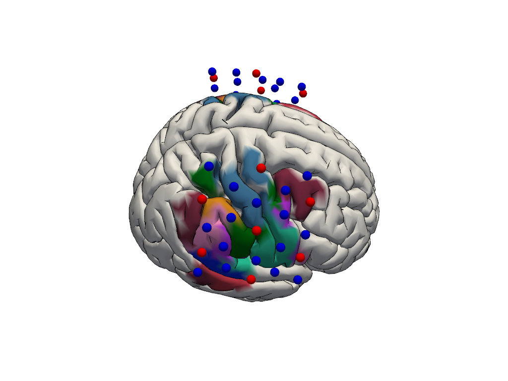
visualize results
[13]:
# plots a surface plot of dOD with axes "channel" and "parcel" using the log of the
# values in dOD on the z-axis for both wavelengths 760 and 850
fig, axes = p.subplots(1, 2, figsize=(12, 6))

for i, wl in enumerate([760.0, 850.0]):
    ax = axes[i]
    im = ax.imshow(np.log10(parcel_dOD.sel(wavelength=wl).values), aspect="auto")
    im.set_clim(-10, 0)
    fig.colorbar(im, ax=ax)
    ax.set_xlabel("parcel")
    ax.set_ylabel("channel")
    ax.set_title(f"log(dOD) for wavelength {wl}")

p.tight_layout()
p.show()


# reduce parcel set to plot to the sensitive parcels
# Find mask of rows to update
color = [
    parcel_colors[parcel] if parcel not in dropped_parcels else [1.0, 1.0, 1.0]
    for parcel in head.brain.vertices.parcel.values
]

plt = pv.Plotter()
vbx.plot_surface(plt, head.brain, color=color, silhouette=True)
vbx.camera_at_cog(plt, head.brain, [400,0,400], fit_scene=True)

# add probe
vbx.plot_labeled_points(
    plt, geo3D_snapped.sel(label=geo3D_snapped.label.str.contains("S|D"))
)
plt.show()
/tmp/ipykernel_5386/4292174508.py:7: RuntimeWarning: divide by zero encountered in log10
  im = ax.imshow(np.log10(parcel_dOD.sel(wavelength=wl).values), aspect="auto")
References
[14]:
cedalion.bib.dump_to_notebook()
Methods used
| [1] | Tucker2022 | cedalion.io.snirf.read_snirf | Stephen Tucker, Jay Dubb, Sreekanth Kura, Alexander von Lühmann, Robert Franke, Jörn M. Horschig, Samuel Powell, Robert Oostenveld, Michael Lührs, Édouard Delaire, Zahra M. Aghajan, Hanseok Yun, Meryem A. Yücel, Qianqian Fang, Theodore J. Huppert, Blaise deB. Frederick, Luca Pollonini, David A. Boas, and Robert Luke. Introduction to the shared near infrared spectroscopy format. Neurophotonics, 10(1):013507, 2022. doi:10.1117/1.NPh.10.1.013507. |
| [2] | Huppert2009 | cedalion.sigproc.quality.snr | Theodore J. Huppert, Solomon G. Diamond, Maria A. Franceschini, and David A. Boas. Homer: a review of time-series analysis methods for near-infrared spectroscopy of the brain. Appl. Opt., 48(10):D280–D298, Apr 2009. doi:https://doi.org/10.1364/AO.48.00D280. |
| [3] | Fonov2011 | cedalion.data.get_icbm152_headmodel_files | Vladimir Fonov, Alan C. Evans, Kelly Botteron, C. Robert Almli, Robert C. McKinstry, and D. Louis Collins. Unbiased average age-appropriate atlases for pediatric studies. NeuroImage, 54(1):313–327, January 2011. doi:10.1016/j.neuroimage.2010.07.033. |
| [4] | Fischl2012 | cedalion.data.get_icbm152_headmodel_files | Bruce Fischl. FreeSurfer. NeuroImage, 62(2):774–781, 2012. doi:10.1016/j.neuroimage.2012.01.021. |
| [5] | Schaefer2018 | cedalion.data.get_icbm152_headmodel_files | Alexander Schaefer, Ru Kong, Evan M Gordon, Timothy O Laumann, Xi-Nian Zuo, Avram J Holmes, Simon B Eickhoff, and BT Thomas Yeo. Local-global parcellation of the human cerebral cortex from intrinsic functional connectivity mri. Cerebral cortex, 28(9):3095–3114, 2018. doi:10.1093/cercor/bhx179. |
| [6] | Fang2009 | cedalion.data.get_precomputed_sensitivity | Qianqian Fang and David A Boas. Monte carlo simulation of photon migration in 3d turbid media accelerated by graphics processing units. Optics express, 17(22):20178–20190, 2009. doi:10.1364/OE.17.020178. |
| [7] | Yu2018 | cedalion.data.get_precomputed_sensitivity | Leiming Yu, Fanny Nina-Paravecino, David Kaeli, and Qianqian Fang. Scalable and massively parallel monte carlo photon transport simulations for heterogeneous computing platforms. Journal of biomedical optics, 23(1):010504–010504, 2018. doi:10.1117/1.JBO.23.1.010504. |
| [8] | Yan2020 | cedalion.data.get_precomputed_sensitivity | Shijie Yan and Qianqian Fang. Hybrid mesh and voxel based monte carlo algorithm for accurate and efficient photon transport modeling in complex bio-tissues. Biomedical Optics Express, 11(11):6262–6270, 2020. doi:10.1364/BOE.409468. |
| [9] | Prahl1998 | cedalion.nirs.common.get_extinction_coefficients | Scott A. Prahl. Optical absorption of hemoglobin. Oregon Medical Laser Center, online resource, 1998. URL: https://omlc.org/spectra/hemoglobin/. |