Photogrammetric Optode Coregistration
Photogrammetry offers a possibility to get subject-specific optode coordinates. This notebook illustrates the individual steps to obtain these coordinates from a textured triangle mesh and a predefined montage.
[1]:
# This cells setups the environment when executed in Google Colab.
try:
    import google.colab
    !curl -s https://raw.githubusercontent.com/ibs-lab/cedalion/dev/scripts/colab_setup.py -o colab_setup.py
    # Select branch with --branch "branch name" (default is "dev")
    %run colab_setup.py
except ImportError:
    pass
[2]:
import logging

import matplotlib.image as mpimg
import matplotlib.pyplot as plt

import numpy as np
import pyvista as pv
import xarray as xr

import cedalion
import cedalion.dataclasses as cdc
import cedalion.data
import cedalion.geometry.registration
import cedalion.io
import cedalion.vis
import cedalion.vis.blocks as vbx
from cedalion.vis.anatomy import OptodeSelector
from cedalion.geometry.photogrammetry.processors import (
    ColoredStickerProcessor,
    geo3d_from_scan,
)
from cedalion.geometry.registration import find_spread_points


xr.set_options(display_expand_data=False)

logging.basicConfig()
logging.getLogger("cedalion").setLevel(logging.DEBUG)
logging.getLogger('trame_client').setLevel(logging.WARNING)
logging.getLogger('trame_server').setLevel(logging.WARNING)
0. Choose between interactive and static mode
This example notebook provides two modes, controlled by the constant INTERACTIVE:
a static mode intended for rendering the documentation
an interactive mode, in which the 3D visualizations react to user input. The camera position can be changed. More importantly, the optode and landmark picking needs these interactive plots.
[3]:
INTERACTIVE = False

if INTERACTIVE:
    # option 1: render in the browser
    # pv.set_jupyter_backend("client")
    # option 2: offload rendering to a server process using trame
    pv.set_jupyter_backend("server")
else:
    pv.set_jupyter_backend("static")  # static rendering (for documentation page)
1. Loading the triangulated surface mesh
Use cedalion.io.read_einstar_obj to read the textured triangle mesh produced by the Einstar scanner. By default we use an example dataset. By setting the fname_ variables the notebook can operate on another scan.
[4]:
# insert here your own files if you do not want to use the example
fname_scan = ""  # path to .obj scan file
fname_snirf = "" # path to .snirf file for montage information
fname_montage_img = "" # path to an image file of the montage

if not fname_scan:
    fname_scan, fname_snirf, fname_montage_img = (
        cedalion.data.get_photogrammetry_example_scan()
    )

surface_mesh = cedalion.io.read_einstar_obj(fname_scan)
display(surface_mesh)
TrimeshSurface(faces: 869980 vertices: 486695 crs: digitized units: millimeter vertex_coords: [])
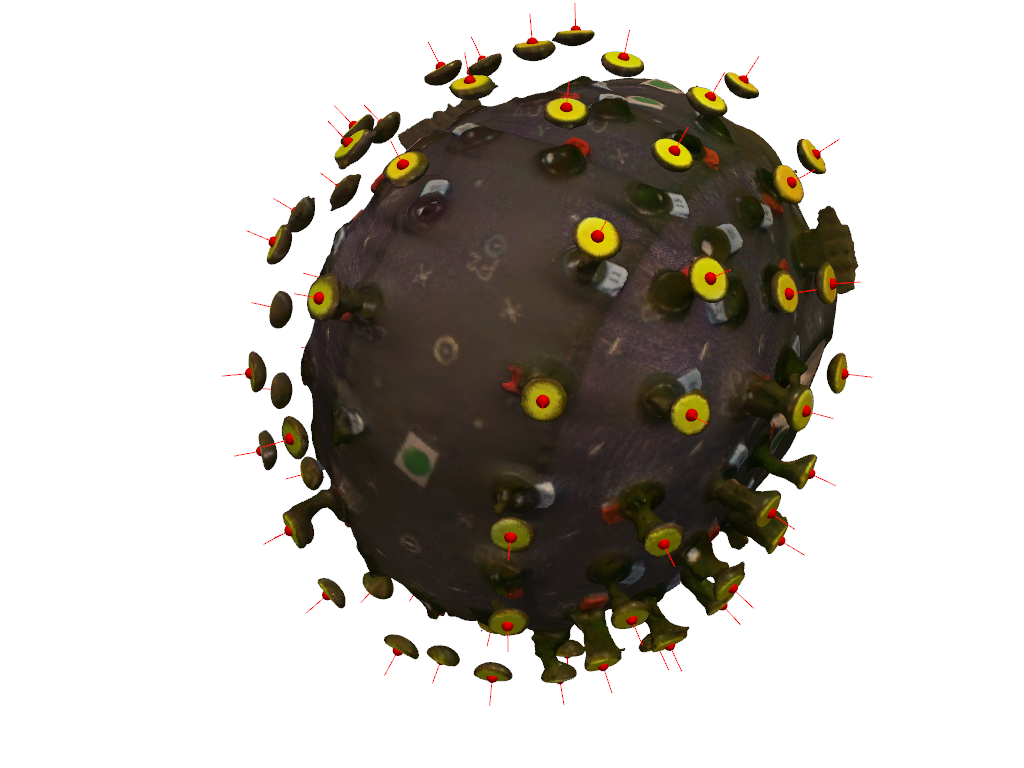
2. Identifying sticker vertices
Processors are meant to analyze the textured mesh and extract positions. The ColoredStickerProcessor searches for colored vertices that form circular areas. We operate in HSV color space and the colors must be specified by their ranges in hue and value. These can be found by usig a color pipette tool on the texture file.
Multiple classes with different colors can be specified. In the following only yellow stickers for class “O(ptode)” are searched. But it could be extended to search also for differently colored sticker. (e.g. “L(andmark)”).
For each sticker the center and the normal is derived. Labels are generated from the class name and a counter, e.g. “O-01, O-02, …”
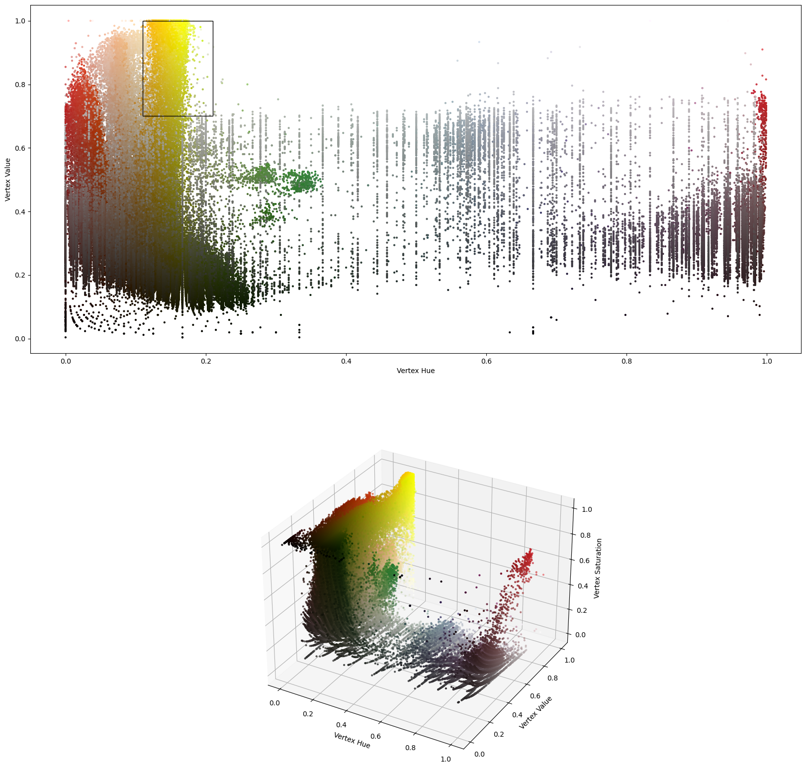
The processor can visualize the scan’s vertex colors before running sticker detection.
The following scatter plot shows the vertex colors in the hue-value plane in which the vertex classification operates. This helps to choose suitable color ranges before calling process().
The black rectangles illustrate the current classification criteria.
[5]:
processor = ColoredStickerProcessor(
    colors={
        "O" : ((0.11, 0.21, 0.7, 1)), # (hue_min, hue_max, value_min, value_max)
        #"L" : ((0.25, 0.37, 0.35, 0.6))
    }
)

preview_details = processor.inspect_colors(surface_mesh)
preview_details.plot_vertex_colors()

sticker_centers, normals, details = processor.process(surface_mesh, details=True)
display(sticker_centers)

DEBUG:cedalion:found 64 clusters.
DEBUG:cedalion:22 vertices belong to no cluster.
DEBUG:cedalion:O - 0: 674 vertices
DEBUG:cedalion:O - 1: 612 vertices
DEBUG:cedalion:O - 2: 538 vertices
[[ 89.200134   6.045319 647.938599]
 [ 89.200134   5.245316 647.979248]
 [ 91.200134   8.845306 647.925781]
 ...
 [124.331436  49.604759 453.649017]
 [122.423584  49.688946 453.390503]
 [124.424706  48.602425 456.144684]]
[[ 91.200134   8.845306 647.925781]
 [ 89.600143   3.965302 647.806641]
 [ 90.320129   3.245316 647.687866]
 ...
 [ 34.000137 -95.936989 536.323303]
 [ 34.80014  -96.269691 536.323303]
 [ 34.400146 -96.094498 536.323303]]
O (0.11, 0.21, 0.7, 1)
DEBUG:cedalion:O - 3: 526 vertices
DEBUG:cedalion:O - 4: 432 vertices
DEBUG:cedalion:O - 5: 347 vertices
DEBUG:cedalion:O - 6: 327 vertices
DEBUG:cedalion:O - 7: 419 vertices
DEBUG:cedalion:O - 8: 450 vertices
DEBUG:cedalion:O - 9: 436 vertices
DEBUG:cedalion:O - 10: 385 vertices
DEBUG:cedalion:O - 11: 592 vertices
DEBUG:cedalion:O - 12: 439 vertices
DEBUG:cedalion:O - 13: 588 vertices
DEBUG:cedalion:O - 14: 360 vertices
DEBUG:cedalion:O - 15: 391 vertices
DEBUG:cedalion:O - 16: 451 vertices
DEBUG:cedalion:O - 17: 408 vertices
DEBUG:cedalion:O - 18: 361 vertices
DEBUG:cedalion:O - 19: 309 vertices
DEBUG:cedalion:O - 20: 400 vertices
DEBUG:cedalion:O - 21: 341 vertices
DEBUG:cedalion:O - 22: 428 vertices
DEBUG:cedalion:O - 23: 400 vertices
DEBUG:cedalion:O - 24: 319 vertices
DEBUG:cedalion:O - 25: 394 vertices
DEBUG:cedalion:O - 26: 552 vertices
DEBUG:cedalion:O - 27: 455 vertices
DEBUG:cedalion:O - 28: 545 vertices
DEBUG:cedalion:O - 29: 456 vertices
DEBUG:cedalion:O - 30: 462 vertices
DEBUG:cedalion:O - 31: 529 vertices
DEBUG:cedalion:O - 32: 491 vertices
DEBUG:cedalion:O - 33: 467 vertices
DEBUG:cedalion:O - 34: 381 vertices
DEBUG:cedalion:O - 35: 406 vertices
DEBUG:cedalion:O - 36: 448 vertices
DEBUG:cedalion:O - 37: 341 vertices
DEBUG:cedalion:O - 38: 274 vertices
DEBUG:cedalion:O - 39: 469 vertices
DEBUG:cedalion:O - 40: 419 vertices
DEBUG:cedalion:O - 41: 444 vertices
DEBUG:cedalion:O - 42: 562 vertices
DEBUG:cedalion:O - 43: 446 vertices
DEBUG:cedalion:O - 44: 393 vertices
DEBUG:cedalion:O - 45: 431 vertices
DEBUG:cedalion:skipping cluster 46 because of too few vertices (7 < 50).
DEBUG:cedalion:O - 47: 436 vertices
DEBUG:cedalion:O - 48: 655 vertices
DEBUG:cedalion:O - 49: 524 vertices
DEBUG:cedalion:O - 50: 309 vertices
DEBUG:cedalion:O - 51: 400 vertices
DEBUG:cedalion:O - 52: 418 vertices
DEBUG:cedalion:O - 53: 570 vertices
DEBUG:cedalion:O - 54: 458 vertices
DEBUG:cedalion:O - 55: 322 vertices
DEBUG:cedalion:O - 56: 566 vertices
DEBUG:cedalion:O - 57: 598 vertices
DEBUG:cedalion:skipping cluster 58 because of too few vertices (11 < 50).
DEBUG:cedalion:O - 59: 367 vertices
DEBUG:cedalion:O - 60: 573 vertices
DEBUG:cedalion:O - 61: 433 vertices
DEBUG:cedalion:O - 62: 263 vertices
[0.51869679 0.52571218 0.09720632 0.09024364 0.0031426  0.26716014
 0.15729909 0.15603078 0.18434642 0.21127269 0.6031898  0.15173879
 0.13589549 0.5367809  0.08970815 0.43860341 0.24223317 0.22831593
 0.11666005 0.38538707 0.06208547 0.26157969 0.21756175 0.33913646
 0.18674489 0.1367986  0.19878102 0.00108876 0.41054799 0.15589406
 0.11664845 0.2340569  0.15650441 0.19405528 0.25735362 0.276244
 0.02862721 0.35069713 0.51928721 0.2630901  0.0427068  0.27555675
 0.20007741 0.29776479 0.09225413 0.21428844 0.05078502 0.29102101
 0.35556447 0.81571727 0.09213511 0.31188405 0.34762441 0.0583965
 0.97653422 0.14968739 0.19396413 0.22924693 0.59414052 0.22320201
 0.79269725]
6.004194440998015
surface.crs digitized
<xarray.DataArray (label: 61, digitized: 3)> Size: 1kB
[mm] 168.2 -1.85 604.7 72.76 -29.73 641.0 ... -89.01 501.7 203.5 -9.854 514.2
Coordinates:
  * label    (label) <U4 976B 'O-28' 'O-05' 'O-37' ... 'O-61' 'O-50' 'O-55'
    type     (label) object 488B PointType.UNKNOWN ... PointType.UNKNOWN
    group    (label) <U1 244B 'O' 'O' 'O' 'O' 'O' 'O' ... 'O' 'O' 'O' 'O' 'O'
Dimensions without coordinates: digitizedVisualize the surface and extraced results.
[6]:
camera_pos = sticker_centers.mean("label").pint.dequantify() - np.array([-500,0,0])
camera_focal_point = sticker_centers.mean("label").pint.dequantify()
camera_up = (0., 0. ,1.)

pvplt = pv.Plotter()
vbx.plot_surface(pvplt, surface_mesh, opacity=1.0)
vbx.plot_labeled_points(pvplt, sticker_centers, color="r")
vbx.plot_vector_field(pvplt, sticker_centers, normals)

pvplt.camera.position = camera_pos
pvplt.camera.focal_point = camera_focal_point
pvplt.camera.up = camera_up

pvplt.show()
The details object is a container for debuging information. It also provides plotting functionality.
The following scatter plot shows the vertex colors in the hue-value plane in which the vertex classification operates.
The black rectangle illustrates the classification criterion.
[7]:
details.plot_vertex_colors()
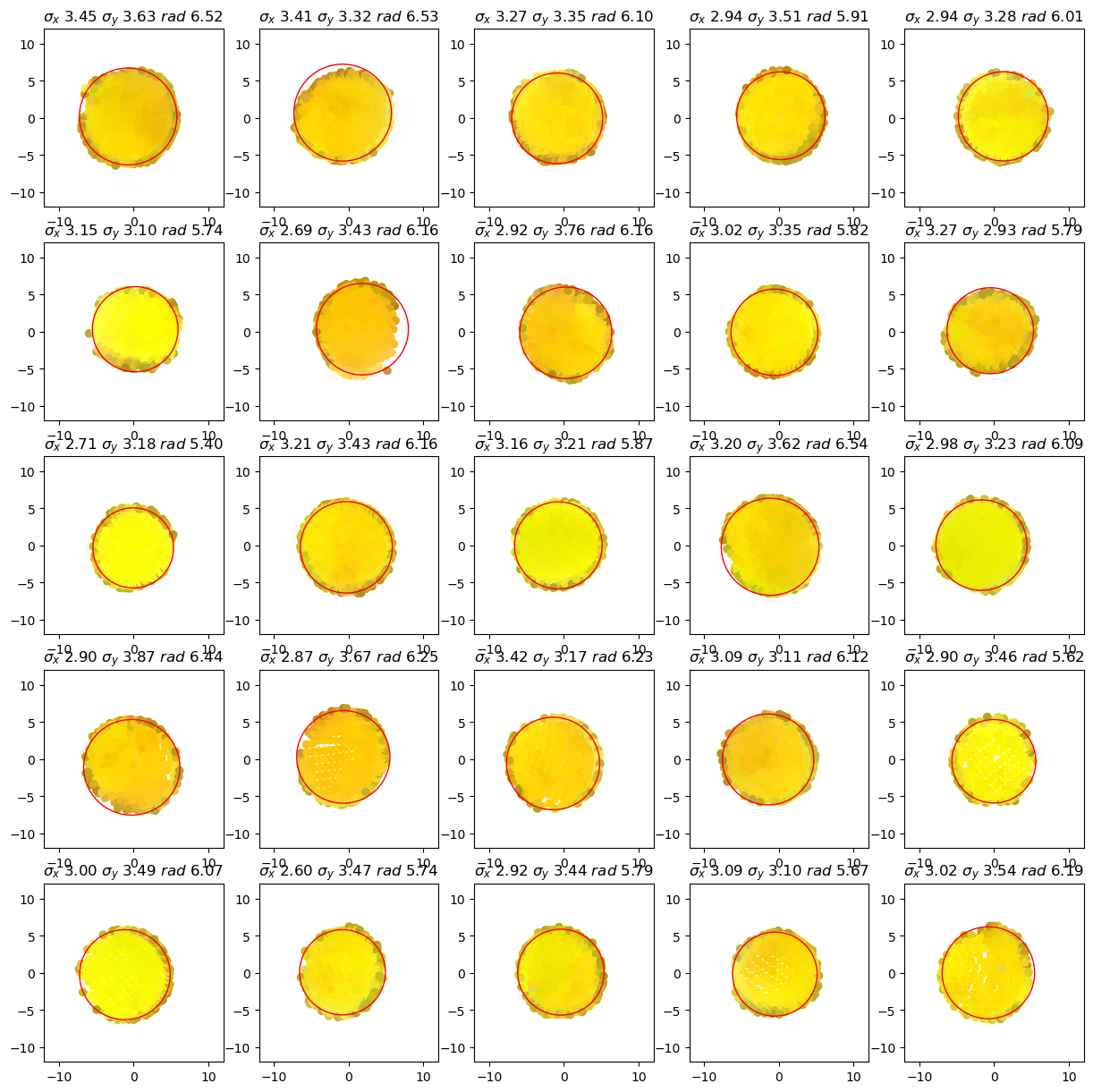
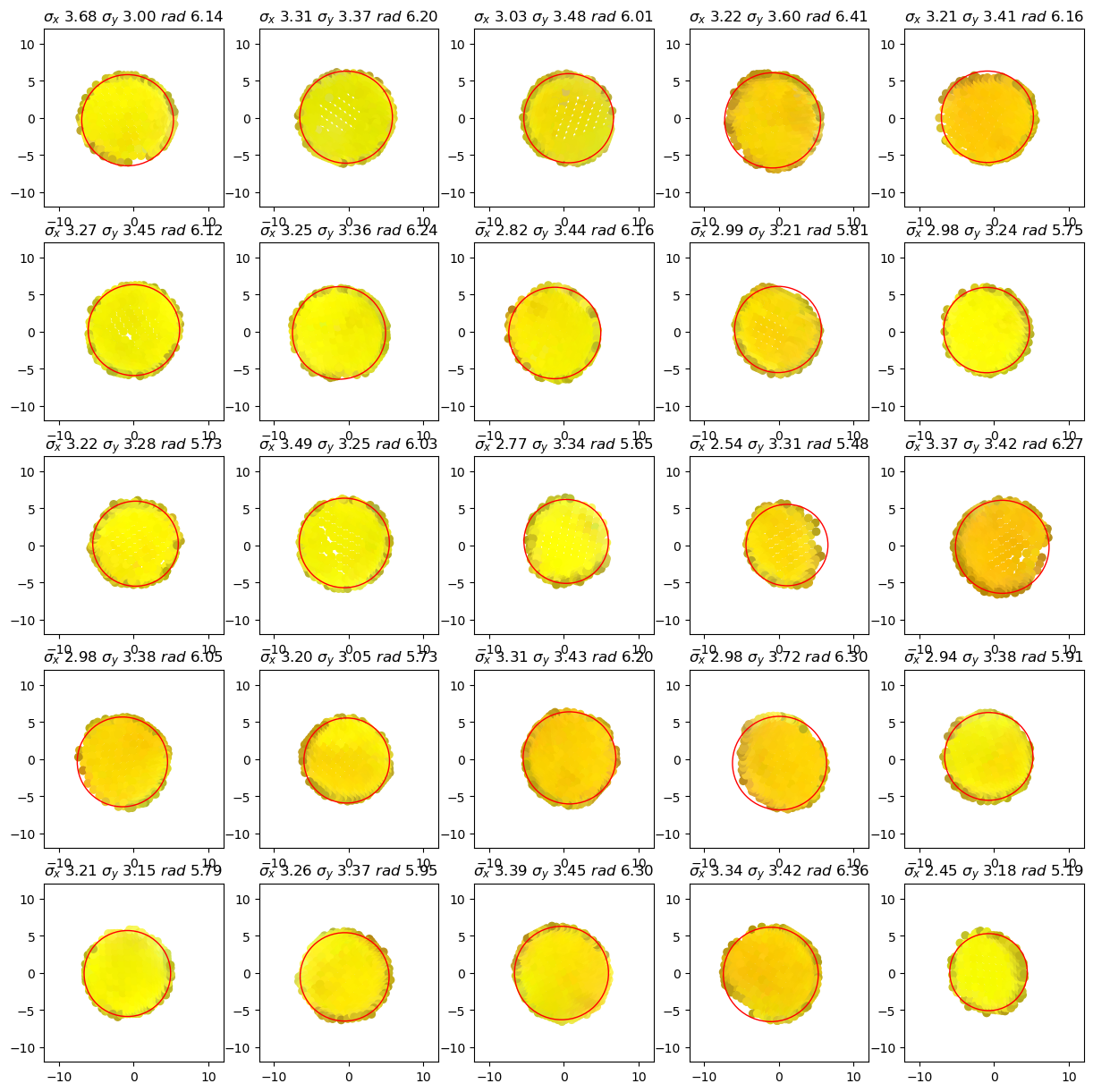
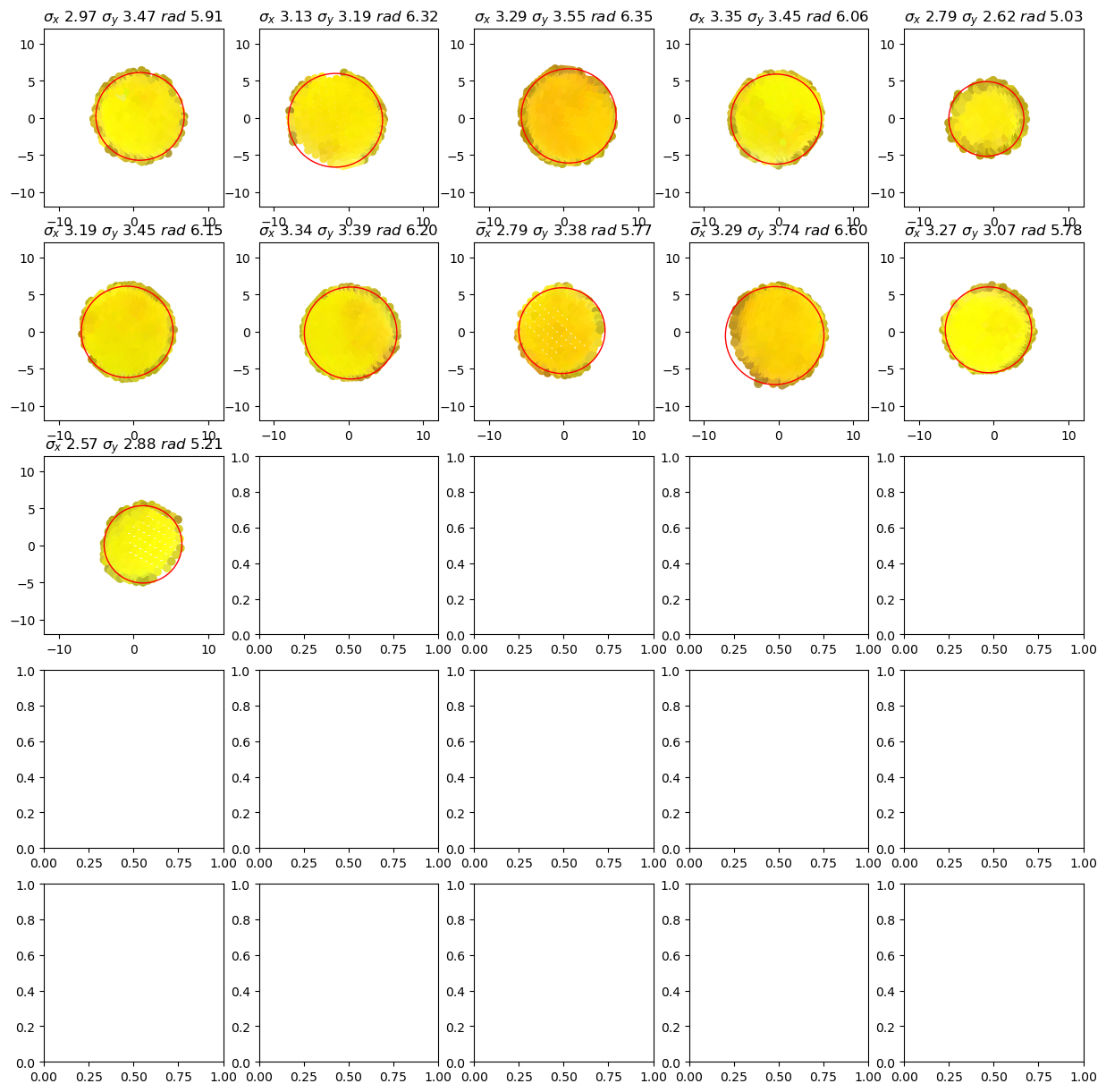
The following plots show for each cluster (tentative group of sticker vertices) The vertex positions perpendicular to the sticker normal as well as the minimum enclosing circle which is used to find the sticker’s center.
[8]:
details.plot_cluster_circles()
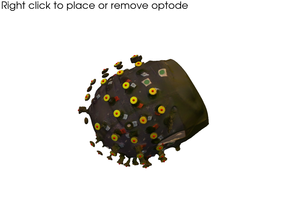
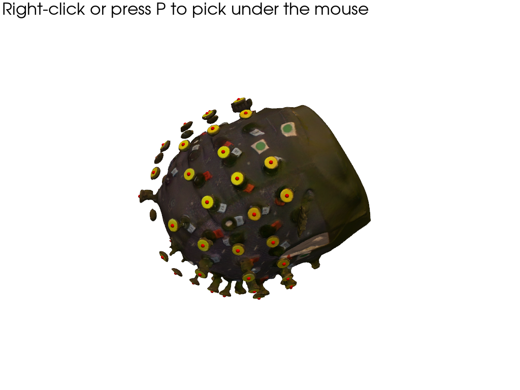
3. Manual corrections of sticker detection
If not all optodes were found automatically, there’s way to remove or add them manually.
The OptodeSelect class provides an interactive visualization of the head scan and the detected stickers (red spheres):
By clicking with the right mouse button on:
a sphere, a misidentified sticker can be removed.
somewhere on the surface, a new sticker position can be added.
[9]:
optode_selector = OptodeSelector(surface_mesh, sticker_centers, normals)
optode_selector.plot()
optode_selector.enable_picking()
vbx.plot_surface(optode_selector.plotter, surface_mesh, opacity=1.0)

optode_selector.plotter.show()
Interactions modify the optode_selector.points and optode_selector.normals. After selecting all optodes, update sticker_centers and normals:
[10]:
sticker_centers = optode_selector.points
normals = optode_selector.normals
display(sticker_centers)
<xarray.DataArray (label: 61, digitized: 3)> Size: 1kB
[mm] 168.2 -1.85 604.7 72.76 -29.73 641.0 ... -89.01 501.7 203.5 -9.854 514.2
Coordinates:
  * label    (label) <U4 976B 'O-28' 'O-05' 'O-37' ... 'O-61' 'O-50' 'O-55'
    type     (label) object 488B PointType.UNKNOWN ... PointType.UNKNOWN
    group    (label) <U1 244B 'O' 'O' 'O' 'O' 'O' 'O' ... 'O' 'O' 'O' 'O' 'O'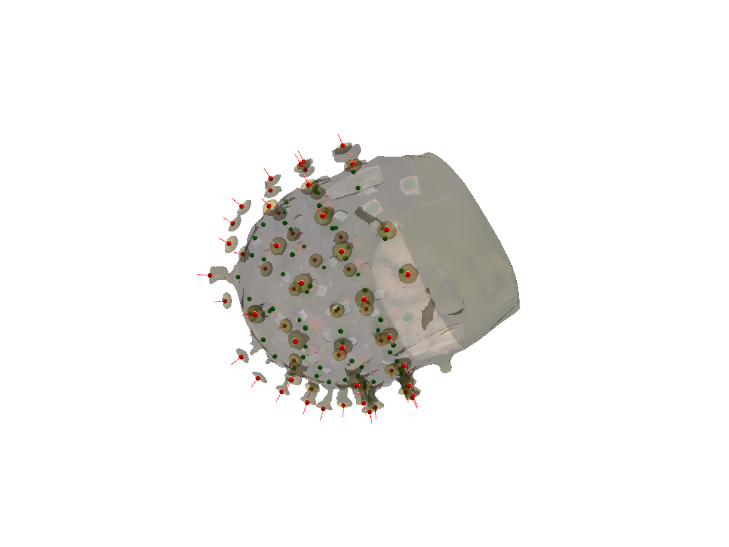
Dimensions without coordinates: digitized4. Project from sticker to scalp surface
Finally, to get from the sticker centers to the scalp coordinates we have to subtract the known lenght of the optodes in the direction of the normals:
[11]:
optode_length = 22.6 * cedalion.units.mm

scalp_coords = sticker_centers.copy()
mask_optodes = sticker_centers.group == "O"
scalp_coords[mask_optodes] = (
    sticker_centers[mask_optodes] - optode_length * normals[mask_optodes]
)
# we make a copy of this raw set of scalp coordinates to use later in the 2nd case of
# the coregistration example that showcases an alternative route if landmark-based
# coregistration fails
scalp_coords_altcase = scalp_coords.copy()

display(scalp_coords)
<xarray.DataArray (label: 61, digitized: 3)> Size: 1kB
[mm] 152.5 -3.156 588.5 70.89 -19.87 620.8 ... -70.83 507.3 181.5 -9.023 519.2
Coordinates:
  * label    (label) <U4 976B 'O-28' 'O-05' 'O-37' ... 'O-61' 'O-50' 'O-55'
    type     (label) object 488B PointType.UNKNOWN ... PointType.UNKNOWN
    group    (label) <U1 244B 'O' 'O' 'O' 'O' 'O' 'O' ... 'O' 'O' 'O' 'O' 'O'
Dimensions without coordinates: digitizedVisualize sticker centers (red) and scalp coordinates (green).
[12]:
pvplt = pv.Plotter()
vbx.plot_surface(pvplt, surface_mesh, opacity=0.3)
vbx.plot_labeled_points(pvplt, sticker_centers, color="r")
vbx.plot_labeled_points(pvplt, scalp_coords, color="g")
vbx.plot_vector_field(pvplt, sticker_centers, normals)
pvplt.show()
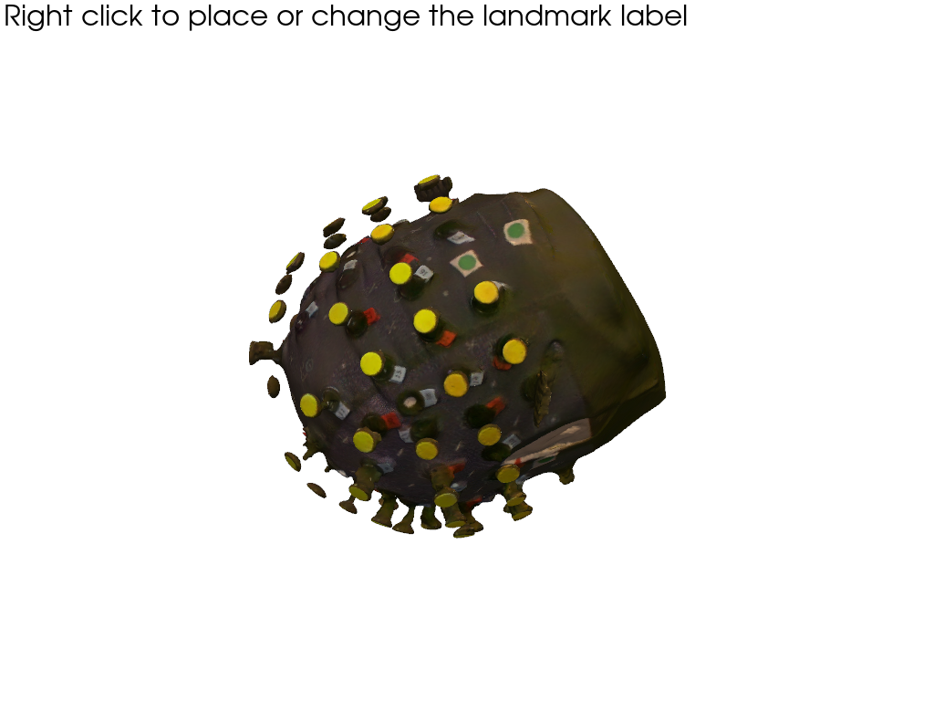
5. Specify landmarks on scanned head surface
5.1. Pick positions in interactive plot
When using the plot_surface function with parameter pick_landmarks set to True, the plot becomes interactive and allows picking the positions of 5 landmarks. These are “Nz”, “Iz”, “Cz”, “Lpa”, “RpA”. If other landmarks need to be picked, pass their labels as a list to pick_landmarks (instead of passing True).
After clicking on the mesh, a green sphere marks the picked location. The sphere has a label attached. If this label is not visible, try to zoom further into the plot (mouse wheel). By clicking again with right mouse button on the sphere one can cycle through the different labels or remove a misplaced landmark.
It helps to add colored markers at the landmark positions when preparing the subject. Here, green stickers were used.
[13]:
pvplt = pv.Plotter()
get_landmarks = vbx.plot_surface(pvplt, surface_mesh, opacity=1.0, pick_landmarks=True)
pvplt.show()
5.2. Retrieve picked positions from interactive plot
The plot_surface function returns a function get_landmarks. Call this function to obtain:
1st value - coordinates of picked landmarks
2nd - labels of corresponding landmarks
[14]:
if INTERACTIVE:
    landmarks = get_landmarks()
else:
    # For documentation purposes and to enable automatically rendered example notebooks
    # we provide the hand-picked coordinates here, too.
    landmark_labels = ["Nz", "Iz", "Cz", "Lpa", "Rpa"]
    landmark_coordinates = np.asarray(
        [
            [14.00420712, -7.84856869, 449.77840004],
            [99.09920059, 29.72154755, 620.73876117],
            [161.63815139, -48.49738938, 494.91210993],
            [82.8771277, 79.79500128, 498.3338802],
            [15.17214095, -60.56186128, 563.29621021],
        ]
    )

    # Wrap landmark positions and labels in a xarray.DataArray structure
    landmarks = xr.DataArray(
        np.vstack(landmark_coordinates),
        dims=["label", "digitized"],
        coords={
            "label": ("label", landmark_labels),
            "type": ("label", [cdc.PointType.LANDMARK] * 5),
            "group": ("label", ["L"] * 5),
        },
    ).pint.quantify("mm")

display(landmarks)
<xarray.DataArray (label: 5, digitized: 3)> Size: 120B
[mm] 14.0 -7.849 449.8 99.1 29.72 620.7 ... 82.88 79.8 498.3 15.17 -60.56 563.3
Coordinates:
  * label    (label) <U3 60B 'Nz' 'Iz' 'Cz' 'Lpa' 'Rpa'
    type     (label) object 40B PointType.LANDMARK ... PointType.LANDMARK
    group    (label) <U1 20B 'L' 'L' 'L' 'L' 'L'
Dimensions without coordinates: digitized6. Mapping the scanned optode positions to a predefined montage.
So far the optode positions found in the photogrammetric head scan carry only generic labels. In oder to identify them, they must be matched with a definition of the actual montage.
Snirf files store next to the actual time series data also the probe geometry, i.e. 3D coordinates of each source and detector. To label the optodes found in the photogrammetric scan, we map each optode to its counterpart in the snirf file.
The snirf coordinates are written during the data acquisition and are typically obtained by arranging the montage on a template head like ICBM-152 or colin27. So despite their similarity, the probe geometries in the snirf file and those from the head scan have differences because of different head geometries aand different coordinate systems.
6.1 Load the montage information from .snirf file
[15]:
# read the example snirf file. Specify a name for the coordinate reference system.
rec = cedalion.io.read_snirf(fname_snirf, crs="aligned")[0]

# read 3D coordinates of the optodes
montage_elements = rec.geo3d

# landmark labels must match exactly. Adjust case where they don't match.
montage_elements = montage_elements.points.rename({"LPA": "Lpa", "RPA": "Rpa"})
INFO:root:Loading from file /home/runner/.cache/cedalion/dev/photogrammetry_example_scan.zip.unzip/photogrammetry_example_scan/photogrammetry_example_31x30.snirf
INFO:root:IndexedGroup MeasurementList at /nirs/data1 in /home/runner/.cache/cedalion/dev/photogrammetry_example_scan.zip.unzip/photogrammetry_example_scan/photogrammetry_example_31x30.snirf initalized with 194 instances of <class 'snirf.pysnirf2.MeasurementListElement'>
INFO:root:IndexedGroup Data at /nirs in /home/runner/.cache/cedalion/dev/photogrammetry_example_scan.zip.unzip/photogrammetry_example_scan/photogrammetry_example_31x30.snirf initalized with 1 instances of <class 'snirf.pysnirf2.DataElement'>
INFO:root:IndexedGroup Stim at /nirs in /home/runner/.cache/cedalion/dev/photogrammetry_example_scan.zip.unzip/photogrammetry_example_scan/photogrammetry_example_31x30.snirf initalized with 0 instances of <class 'snirf.pysnirf2.StimElement'>
INFO:root:IndexedGroup Aux at /nirs in /home/runner/.cache/cedalion/dev/photogrammetry_example_scan.zip.unzip/photogrammetry_example_scan/photogrammetry_example_31x30.snirf initalized with 0 instances of <class 'snirf.pysnirf2.AuxElement'>
INFO:root:IndexedGroup Nirs at / in /home/runner/.cache/cedalion/dev/photogrammetry_example_scan.zip.unzip/photogrammetry_example_scan/photogrammetry_example_31x30.snirf initalized with 1 instances of <class 'snirf.pysnirf2.NirsElement'>
WARNING:cedalion:generating generic source labels
WARNING:cedalion:generating generic detector labels
WARNING:cedalion:landmark labels were provided but not their positions. Removing labels
WARNING:cedalion:generating generic source labels
WARNING:cedalion:generating generic detector labels
WARNING:cedalion:generating generic source labels
WARNING:cedalion:generating generic detector labels
WARNING:cedalion:generating generic source labels
WARNING:cedalion:generating generic detector labels
INFO:root:Closing Snirf file /home/runner/.cache/cedalion/dev/photogrammetry_example_scan.zip.unzip/photogrammetry_example_scan/photogrammetry_example_31x30.snirf
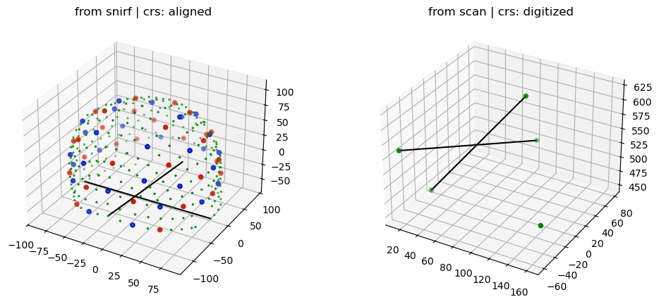
6.2 Find a transformation to align selected landmarks to montage coordinates
The coordinates in the snirf file and from the photogrammetric scan use different coordinate reference systems (CRS). In Cedalion the user needs to explicitly name different CRSs. Here the labels ‘digitized’ and ‘aligned’ were used.
The following plot shows the probe geometry from the snirf file and the landmarks from the head scan. Two black lines Nz-Iz and Lpa-Rpa are added to guide the eye.
[16]:
f = plt.figure(figsize=(12,5))
ax1 = f.add_subplot(1,2,1, projection="3d")
ax2 = f.add_subplot(1,2,2, projection="3d")
colors = {cdc.PointType.SOURCE: "r", cdc.PointType.DETECTOR: "b"}
sizes = {cdc.PointType.SOURCE: 20, cdc.PointType.DETECTOR: 20}

for i, (type, x) in enumerate(montage_elements.groupby("type")):
    x = x.pint.to("mm").pint.dequantify()
    ax1.scatter(x[:, 0], x[:, 1], x[:, 2], c=colors.get(type, "g"), s=sizes.get(type, 2))

for i, (type, x) in enumerate(landmarks.groupby("type")):
    x = x.pint.to("mm").pint.dequantify()
    ax2.scatter(x[:, 0], x[:, 1], x[:, 2], c=colors.get(type, "g"), s=20)

for ax, points in [(ax1, montage_elements), (ax2, landmarks)]:
    points = points.pint.to("mm").pint.dequantify()
    ax.plot([points.loc["Nz",0], points.loc["Iz",0]],
            [points.loc["Nz",1], points.loc["Iz",1]],
            [points.loc["Nz",2], points.loc["Iz",2]],
            c="k"
            )
    ax.plot([points.loc["Lpa",0], points.loc["Rpa",0]],
            [points.loc["Lpa",1], points.loc["Rpa",1]],
            [points.loc["Lpa",2], points.loc["Rpa",2]],
            c="k"
            )

ax1.set_title(f"from snirf | crs: {montage_elements.points.crs}")
ax2.set_title(f"from scan | crs: {landmarks.points.crs}");

Subsequently, to bring the coordinates into the same space, from the landmarks a transformation (translations and rotations) is derived. This transforms the coordinates from the snirf file to the CRS of the photogramettric scan.
The following plot illustrates the transformed coordinates of sources (red) and detectors (blue). Deviations between these coordinates and the head surface are expected, since the optode positions where specified on a different head geometry.
[17]:
trafo = cedalion.geometry.registration.register_trans_rot(landmarks, montage_elements)

filtered_montage_elements = montage_elements.where(
    (montage_elements.type == cdc.PointType.SOURCE)
    | (montage_elements.type == cdc.PointType.DETECTOR),
    drop=True,
)
filtered_montage_elements_t = filtered_montage_elements.points.apply_transform(trafo)

pvplt = pv.Plotter()
vbx.plot_surface(pvplt, surface_mesh, color="w", opacity=.2)
vbx.plot_labeled_points(pvplt, filtered_montage_elements_t)
pvplt.show()
6.3 Iterative closest point algorithm to find labels for detected optode centers
Finally, the mapping is derived by iteratively trying to find a transformation that yilds the best match between the snirf and the scanned coordinates.
The following plot visualizes the result:
Green points represent optode centers
Next to them there shall be labels assumed by ICP algorithm (show_labels = True)
[18]:
# iterative closest point registration
idx = cedalion.geometry.registration.icp_with_full_transform(
    scalp_coords, filtered_montage_elements_t, max_iterations=100
)

# extract labels for detected optodes
label_dict = {}
for i, label in enumerate(filtered_montage_elements.coords["label"].values):
    label_dict[i] = label
labels = [label_dict[index] for index in idx]

# write labels to scalp_coords
scalp_coords = scalp_coords.assign_coords(label=labels)

# add landmarks
geo3Dscan = geo3d_from_scan(scalp_coords, landmarks)

display(geo3Dscan)
<xarray.DataArray (label: 66, digitized: 3)> Size: 2kB
[mm] 152.5 -3.156 588.5 70.89 -19.87 620.8 ... 79.8 498.3 15.17 -60.56 563.3
Coordinates:
    type     (label) object 528B PointType.SOURCE ... PointType.LANDMARK
    group    (label) <U1 264B 'O' 'O' 'O' 'O' 'O' 'O' ... 'L' 'L' 'L' 'L' 'L'
  * label    (label) <U3 792B 'S21' 'S23' 'D13' 'D8' ... 'Iz' 'Cz' 'Lpa' 'Rpa'
Dimensions without coordinates: digitized
Attributes: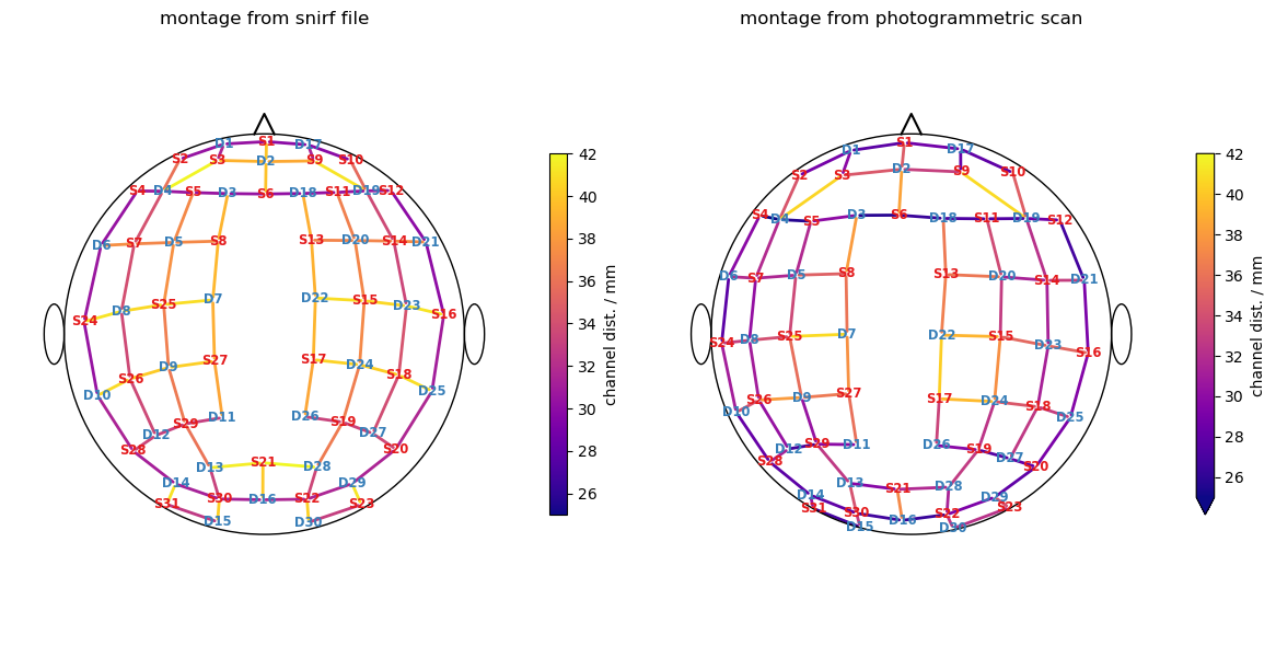
units: mm[19]:
f,ax = plt.subplots(1,2, figsize=(12,6))
cedalion.vis.anatomy.scalp_plot(
    rec["amp"],
    montage_elements,
    cedalion.nirs.channel_distances(rec["amp"], montage_elements),
    ax=ax[0],
    optode_labels=True,
    cb_label="channel dist. / mm",
    cmap="plasma",
    vmin=25,
    vmax=42,
)
ax[0].set_title("montage from snirf file")
cedalion.vis.anatomy.scalp_plot(
    rec["amp"],
    geo3Dscan,
    cedalion.nirs.channel_distances(rec["amp"], geo3Dscan),
    ax=ax[1],
    optode_labels=True,
    cb_label="channel dist. / mm",
    cmap="plasma",
    vmin=25,
    vmax=42,
)
ax[1].set_title("montage from photogrammetric scan")
plt.tight_layout()
WARNING:matplotlib.axes._base:Ignoring fixed y limits to fulfill fixed data aspect with adjustable data limits.
WARNING:matplotlib.axes._base:Ignoring fixed y limits to fulfill fixed data aspect with adjustable data limits.
WARNING:matplotlib.axes._base:Ignoring fixed x limits to fulfill fixed data aspect with adjustable data limits.
WARNING:matplotlib.axes._base:Ignoring fixed x limits to fulfill fixed data aspect with adjustable data limits.
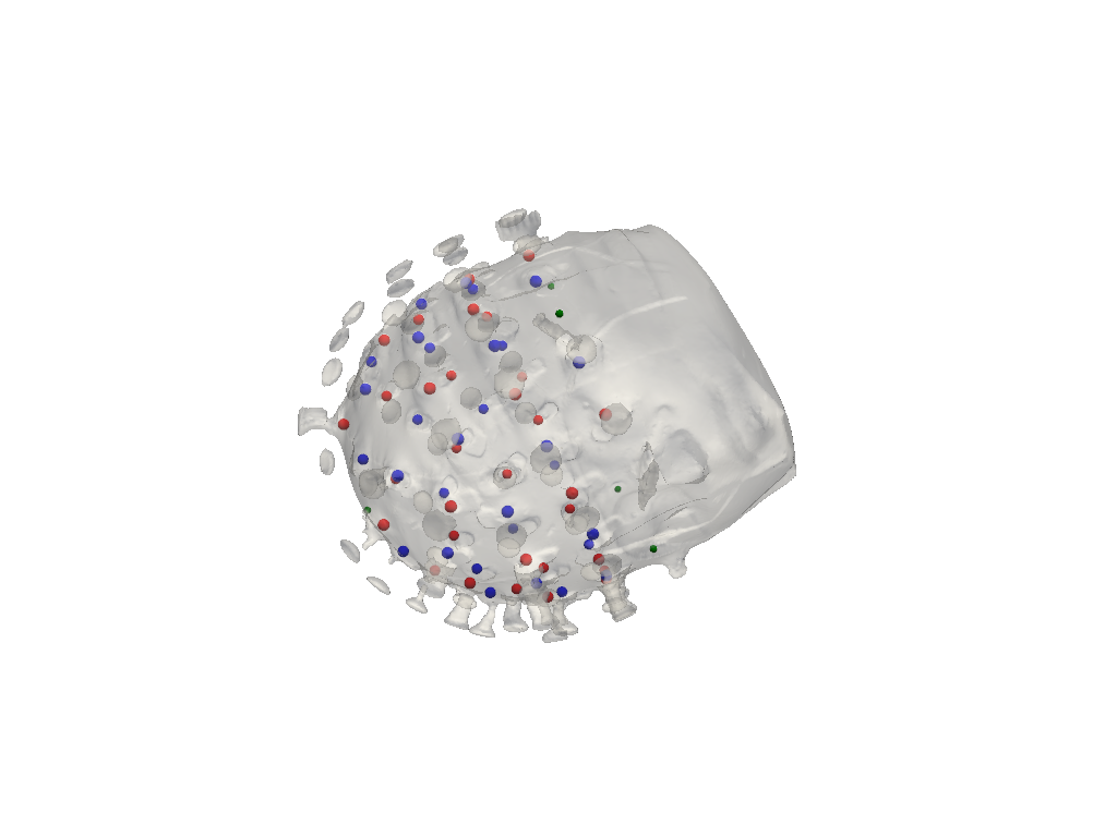
Visualization of successfull assignment (show_labels = True)
[20]:
pvplt = pv.Plotter()
cedalion.vis.anatomy.plot_brain_and_scalp(None, surface_mesh.mesh, None, None, plotter=pvplt)
vbx.plot_labeled_points(pvplt, geo3Dscan, show_labels=True)
pvplt.show()

6.4 Alternative approach without landmarks
Mapping the optode labels can fail for example because of a bad landmark selection.
In such cases it is possible to find a new transformation by manually labeling three optodes. This is done by selecting them in a given order. For that it helps to have a visualization of the montage of your experiment.
[21]:
if fname_montage_img:
    # Load and display the image
    img = mpimg.imread(fname_montage_img)
    plt.figure(figsize=(12, 10))
    plt.imshow(img)
    plt.axis("off")  # Turn off axis labels and ticks
    plt.show()
else:
    print("No montage image specified.")
Search for three optodes that are evenly spreaded across the head surface. Afterwards prompt the uer to right click on each of them.
[22]:
spread_point_labels = find_spread_points(filtered_montage_elements)
print("Select those points")
print(spread_point_labels)

points = []
pvplt = pv.Plotter()
vbx.plot_surface(pvplt, surface_mesh, opacity=1.0)
vbx.plot_labeled_points(pvplt, sticker_centers, color="r", ppoints = points)
pvplt.show()
/home/runner/miniconda3/envs/cedalion/lib/python3.11/site-packages/xarray/core/variable.py:315: UnitStrippedWarning: The unit of the quantity is stripped when downcasting to ndarray.
  data = np.asarray(data)
Select those points
['S1' 'D30' 'S31']
Retrieve picked positions:
[23]:
if INTERACTIVE:
    labeled_points = points
else:
    # For documentation purposes and to enable automatically rendered example notebooks
    # we provide the hand-picked coordinates here, too.
    labeled_points = [19, 52, 50]

labeled_points
[23]:
[19, 52, 50]
Write the selected labels to the corresponding points of xarray.DataArray scalp_coords:
[24]:
new_labels = scalp_coords_altcase.label.values.copy()
for i, idx in enumerate(labeled_points):
    new_labels[idx] = spread_point_labels[i]
scalp_coords_altcase = scalp_coords_altcase.assign_coords(label=new_labels)
scalp_coords_altcase
[24]:
<xarray.DataArray (label: 61, digitized: 3)> Size: 1kB
[mm] 152.5 -3.156 588.5 70.89 -19.87 620.8 ... -70.83 507.3 181.5 -9.023 519.2
Coordinates:
    type     (label) object 488B PointType.UNKNOWN ... PointType.UNKNOWN
    group    (label) <U1 244B 'O' 'O' 'O' 'O' 'O' 'O' ... 'O' 'O' 'O' 'O' 'O'
  * label    (label) <U4 976B 'O-28' 'O-05' 'O-37' ... 'O-61' 'O-50' 'O-55'
Dimensions without coordinates: digitizedFind the affine transformation for the newly labeled points and apply it to the montage optodes
[25]:
trafo2 = cedalion.geometry.registration.register_trans_rot(
    scalp_coords_altcase, montage_elements
)

filtered_montage_elements = montage_elements.where(
    (montage_elements.type == cdc.PointType.SOURCE)
    | (montage_elements.type == cdc.PointType.DETECTOR),
    drop=True,
)
filtered_montage_elements_t = filtered_montage_elements.points.apply_transform(trafo2)
and run ICP algorithm for label assignment once again, extract labels for detected optodes and plot the results
[26]:
# iterative closest point registration
idx = cedalion.geometry.registration.icp_with_full_transform(
    scalp_coords_altcase, filtered_montage_elements_t, max_iterations=100
)
# extract labels for detected optodes
label_dict = {}
for i, label in enumerate(filtered_montage_elements.coords["label"].values):
    label_dict[i] = label
labels = [label_dict[index] for index in idx]

# write labels to scalp_coords
scalp_coords_altcase = scalp_coords_altcase.assign_coords(label=labels)

# add landmarks
geo3Dscan_alt = geo3d_from_scan(scalp_coords_altcase, landmarks)
[27]:
f,ax = plt.subplots(1,2, figsize=(12,6))
cedalion.vis.anatomy.scalp_plot(
    rec["amp"],
    montage_elements,
    cedalion.nirs.channel_distances(rec["amp"], montage_elements),
    ax=ax[0],
    optode_labels=True,
    cb_label="channel dist. / mm",
    cmap="plasma",
    vmin=25,
    vmax=42,
)

ax[0].set_title("montage from snirf file")
cedalion.vis.anatomy.scalp_plot(
    rec["amp"],
    geo3Dscan_alt,
    cedalion.nirs.channel_distances(rec["amp"], geo3Dscan_alt),
    ax=ax[1],
    optode_labels=True,
    cb_label="channel dist. / mm",
    cmap="plasma",
    vmin=25,
    vmax=42,
)
ax[1].set_title("montage from photogrammetric scan")
plt.tight_layout()
WARNING:matplotlib.axes._base:Ignoring fixed y limits to fulfill fixed data aspect with adjustable data limits.
WARNING:matplotlib.axes._base:Ignoring fixed y limits to fulfill fixed data aspect with adjustable data limits.
WARNING:matplotlib.axes._base:Ignoring fixed x limits to fulfill fixed data aspect with adjustable data limits.
WARNING:matplotlib.axes._base:Ignoring fixed x limits to fulfill fixed data aspect with adjustable data limits.

References
[28]:
cedalion.bib.dump_to_notebook()
Methods used
| [1] | Tucker2022 | cedalion.io.snirf.read_snirf | Stephen Tucker, Jay Dubb, Sreekanth Kura, Alexander von Lühmann, Robert Franke, Jörn M. Horschig, Samuel Powell, Robert Oostenveld, Michael Lührs, Édouard Delaire, Zahra M. Aghajan, Hanseok Yun, Meryem A. Yücel, Qianqian Fang, Theodore J. Huppert, Blaise deB. Frederick, Luca Pollonini, David A. Boas, and Robert Luke. Introduction to the shared near infrared spectroscopy format. Neurophotonics, 10(1):013507, 2022. doi:10.1117/1.NPh.10.1.013507. |