S1: Head models and Forward Modelling
This notebook introduces how Cedalion handles head models and forward modelling for diffuse optical tomography.
Learning objectives
In this notebook you will learn to:
Understand the
TwoSurfaceHeadModelstructure (segmentation, scalp mesh, brain mesh, landmarks)Navigate the coordinate reference systems used in Cedalion (digitized, ijk, ras/mni)
Build a forward model: register optodes to the scalp, compute fluence, form the sensitivity matrix
[1]:
# This cells setups the environment when executed in Google Colab.
try:
    import google.colab
    !curl -s https://raw.githubusercontent.com/ibs-lab/cedalion/dev/scripts/colab_setup.py -o colab_setup.py
    # Select branch with --branch "branch name" (default is "dev")
    %run colab_setup.py
except ImportError:
    pass
[2]:
from pathlib import Path
from tempfile import TemporaryDirectory

import cedalion
import cedalion.data
import cedalion.dataclasses as cdc
import cedalion.dot
import cedalion.io
import cedalion.nirs
import cedalion.vis.anatomy
import cedalion.vis.blocks as vbx
import matplotlib.pyplot as p
import numpy as np
import pyvista as pv
import xarray as xr
from cedalion import units
from matplotlib.colors import ListedColormap

# set pyvista's jupyter backend to 'server' for interactive 3D plots
pv.set_jupyter_backend("static")
# pv.set_jupyter_backend('server')

xr.set_options(display_expand_data=False);
Configuration
The constants in the next cell control the behavior of the notebook.
[3]:
# set this to either 'colin27', 'icbm152', 'custom_from_segmentation', 'custom_from_surfaces'
HEAD_MODEL = "colin27"

# set this to either 'mcx' or 'nirfaster'
FORWARD_MODEL = "mcx"

# set this to False to actually run the forward model
PRECOMPUTED_SENSITIVITY = True
Create a temporary directory as a working directory.
[4]:
working_directory = TemporaryDirectory()
tmp_dir_path = Path(working_directory.name)
Loading and inspecting an example dataset
This notebook loads one of Cedalion’s example datasets.
Using a function from the cedalion.data package, the following cell will download a snirf file with a recording of a fingertapping experiment.
The content of the snirf file is returned as a cedalion.dataclasses.Recording object.
[5]:
rec = cedalion.data.get_fingertappingDOT()
The Recording container carries time series and related objects through the program in ordered dictionaries much like a segmented tray carrying items in separate compartments.
This notebook mainly needs the probe geometry and channel definitions, detailed below.
Probe Geometry
The snirf file contains the 3D probe geometry. When loaded in Cedalion, the probe geometry is represented in a xarray.DataArray with shape (number of labeled points x 3).
It is available as an attribute of the Recording container:
[6]:
rec.geo3d
[6]:
<xarray.DataArray (label: 346, digitized: 3)> Size: 8kB
[mm] -77.82 15.68 23.17 -61.91 21.23 56.49 ... 14.23 -38.28 81.95 -0.678 -37.03
Coordinates:
    type     (label) object 3kB PointType.SOURCE ... PointType.LANDMARK
  * label    (label) <U6 8kB 'S1' 'S2' 'S3' 'S4' ... 'FFT10h' 'FT10h' 'FTT10h'
Dimensions without coordinates: digitizedThis array stores 3D coordinates for 346 points. The first dimension, named 'label', indexes the points, while the second dimension holds the three coordinate values for each point. In Cedalion, the name of the second dimension serves as the label for the coordinate’s reference system, which in this case is set to 'digitized'.
Two coordinate arrays are linked to 'label' dimension. The 'label' coordinate assigns a string name to each 3D point (for example, 'S1' for the first source or 'Nz' for the nasion). Using values of cedalion.dataclasses.PointType, the 'type' coordinate is used to distinguish between sources, detectors and landmarks.
The values stored in the geo3d array have physical units associated with them. In this case, the coordinates are given in millimeters.
This particular schema of representing geometry information in a xarray.DataArray is used throughout Cedalion. Arrays following this schema are called cedalion.typing.LabeledPoints.
Channel Definitions
This dataset contains one continuous-wave raw amplitudes time series. It is stored in the Recording container within the timeseries dictionary under the key 'amp'.
[7]:
rec.timeseries.keys()
[7]:
odict_keys(['amp'])
Channels are defined by source-detector pairs. Cedalion uses two ways of representing channel definitions: measurement lists and time series coordinates.
In the SNIRF file, channels are specified in measurement lists, a tabular data structure that lists for each channel source, detector, wavelength and data type.
For each loaded time series, the measurement list is stored as a pandas.DataFrame in rec._measurement_lists under the same key.
[8]:
meas_list = rec._measurement_lists["amp"]
display(meas_list)
| sourceIndex | detectorIndex | wavelengthIndex | wavelengthActual | wavelengthEmissionActual | dataType | dataUnit | dataTypeLabel | dataTypeIndex | sourcePower | detectorGain | moduleIndex | sourceModuleIndex | detectorModuleIndex | channel | source | detector | wavelength | chromo | |
|---|---|---|---|---|---|---|---|---|---|---|---|---|---|---|---|---|---|---|---|
| 0 | 1 | 1 | 1 | None | None | 1 | None | raw-DC | 1 | None | None | None | None | None | S1D1 | S1 | D1 | 760.0 | None |
| 1 | 1 | 2 | 1 | None | None | 1 | None | raw-DC | 1 | None | None | None | None | None | S1D2 | S1 | D2 | 760.0 | None |
| 2 | 1 | 4 | 1 | None | None | 1 | None | raw-DC | 1 | None | None | None | None | None | S1D4 | S1 | D4 | 760.0 | None |
| 3 | 1 | 5 | 1 | None | None | 1 | None | raw-DC | 1 | None | None | None | None | None | S1D5 | S1 | D5 | 760.0 | None |
| 4 | 1 | 6 | 1 | None | None | 1 | None | raw-DC | 1 | None | None | None | None | None | S1D6 | S1 | D6 | 760.0 | None |
| ... | ... | ... | ... | ... | ... | ... | ... | ... | ... | ... | ... | ... | ... | ... | ... | ... | ... | ... | ... |
| 195 | 14 | 27 | 2 | None | None | 1 | None | raw-DC | 1 | None | None | None | None | None | S14D27 | S14 | D27 | 850.0 | None |
| 196 | 14 | 28 | 2 | None | None | 1 | None | raw-DC | 1 | None | None | None | None | None | S14D28 | S14 | D28 | 850.0 | None |
| 197 | 14 | 29 | 2 | None | None | 1 | None | raw-DC | 1 | None | None | None | None | None | S14D29 | S14 | D29 | 850.0 | None |
| 198 | 14 | 31 | 2 | None | None | 1 | None | raw-DC | 1 | None | None | None | None | None | S14D31 | S14 | D31 | 850.0 | None |
| 199 | 14 | 32 | 2 | None | None | 1 | None | raw-DC | 1 | None | None | None | None | None | S14D32 | S14 | D32 | 850.0 | None |
200 rows × 19 columns
The 'amp' time series is represented as a xarray.DataArray with dimensions 'channel', 'wavelength' and 'time'. Three coordinate arrays are linked to the 'channel' dimension, specifying for each channel a string label as well as the string label and the corresponding source and detector labels (e.g. the first channel 'S1D1' is between source 'S1' and detector 'D1').
[9]:
rec.timeseries["amp"]
[9]:
<xarray.DataArray (channel: 100, wavelength: 2, time: 8794)> Size: 14MB
[V] 0.0874 0.08735 0.08819 0.08887 0.0879 ... 0.09108 0.09037 0.09043 0.08999
Coordinates:
  * time        (time) float64 70kB 0.0 0.2294 0.4588 ... 2.017e+03 2.017e+03
    samples     (time) int64 70kB 0 1 2 3 4 5 ... 8788 8789 8790 8791 8792 8793
  * channel     (channel) object 800B 'S1D1' 'S1D2' 'S1D4' ... 'S14D31' 'S14D32'
    source      (channel) object 800B 'S1' 'S1' 'S1' 'S1' ... 'S14' 'S14' 'S14'
    detector    (channel) object 800B 'D1' 'D2' 'D4' 'D5' ... 'D29' 'D31' 'D32'
  * wavelength  (wavelength) float64 16B 760.0 850.0
Attributes: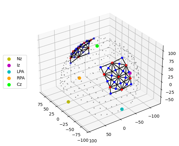
data_type_group: unprocessed rawThe function cedalion.vis.anatomy visualizes the probe geometry. Optode locations are obtained from the geo3d array, while channel definitions are derived from the time series.
Sources, detectors and landmarks are represented as red, blue and grey dots, respectively. The nasion is highlighted in yellow.
[10]:
cedalion.vis.anatomy.plot_montage3D(rec["amp"], rec.geo3d)
Coordinate systems
When working with probe and head model geometries, it is important to distinguish between coordinates from three different coordinate reference systems (CRS):
Digitization space (
CRS='digitized')This is the coordinate space used by the digitization or montage planning tool. In this example, optode positions are given in millimeters with the origin located at the head center and the y-axis pointing in the superior direction. The CRS has the user-configurable name
'digitized'. Other digitization tools may use different names, units or coordinate systems.Voxel space (
CRS='ijk)Tissue masks from segmented MRI scans are in voxel space, where coordinate axes are aligned with voxel edges. Independent of the MRI scanner resolution or the physical voxel size, voxel space is defined such that each voxel has unit edge length and dimensionless coordinates.
Axis-aligned grids are computationally efficient, which is why the photon propagation code MCX uses this coordinate system.
Scanner space / RAS space (
CRS='ras')Scanner space differs from voxel space in that it uses physical units and its coordinate axes point in the Right, Anterior, and Superior directions. Therefore, scanner space is also referred to as RAS space. Both voxel and scanner spaces are related through affine transformations which are stored in the head model as
t_ijk2rasandt_ras2ijk.The scanner space of the standard Colin27 and ICBM-152 heads is widely used as a common coordinate reference system to share results. To highlight this particularly important CRS the head models returned by
get_standard_headmodeluse the label'mni'instead of'ras'for the scanner space.
To avoid confusion between different coordinate systems, Cedalion is explicit about the CRS associated with each point cloud or surface.
As shown above a dimension name of the geo3d array is used to track the CRS. Another way to inspect the CRS is by using the .points accessor:
[11]:
print(f"The coordinate reference system of the probe geometry is '{rec.geo3d.points.crs}'")
The coordinate reference system of the probe geometry is 'digitized'
The TwoSurfaceHeadModel
The forward model simulates photon propagation through different tissue types. Starting from an anatomical MRI scan, tissue segmentation assigns each voxel to a specific tissue type and corresponding optical properties.
The image reconstruction method implemented in Cedalion does not estimate absorption changes for all voxels. Instead, the inverse problem is simplified by defining two surfaces representing the scalp and the brain and by restricting the reconstruction of absorption changes to voxels in their vicinitiy.
The class cedalion.dot.TwoSurfaceHeadModel groups together the segmentation mask, landmark positions and affine transformations as well as the scalp and brain surfaces.
Constructing the TwoSurfaceHeadModel
There are three ways how to construct a TwoSurfaceHeadModel:
using the function
cedalion.dot.get_standard_headmodelfrom tissue segmentation masks. Cedalion derives scalp and brain surfaces.
from tissue segmentation masks and triangulated surface meshes generated by an external tool
[12]:
if HEAD_MODEL in ["colin27", "icbm152"]:
    # use a factory method for the standard head models
    head_ijk = cedalion.dot.get_standard_headmodel(HEAD_MODEL)

elif HEAD_MODEL == "custom_from_segmentation":
    # point these to a directory with segmentation masks
    segm_datadir = Path("/path/to/dir/with/segmentation_masks")
    mask_files = {
        "csf": "mask_csf.nii",
        "gm": "mask_gray.nii",
        "scalp": "mask_skin.nii",
        "skull": "mask_bone.nii",
        "wm": "mask_white.nii",
    }
    # the landmarks must be in scanner (RAS) space.
    # For example Slicer3D can be used to pick the landmarks.
    landmarks_file = Path("/path/to/landmarks.mrk.json")

    # Construct a head model from segmentation mask.
    head_ijk = cedalion.dot.TwoSurfaceHeadModel.from_segmentation(
        segmentation_dir=segm_datadir,
        mask_files=mask_files,
        landmarks_ras_file=landmarks_file,
        # adjust these to control mesh parameters
        brain_face_count=None,
        scalp_face_count=None,
        smoothing=0.0,
    )
elif HEAD_MODEL == "custom_from_surfaces":
    # point these to a directory with segmentation masks
    segm_datadir = Path("/path/to/dir/with/segmentation_masks")
    mask_files = {
        "csf": "mask_csf.nii",
        "gm": "mask_gray.nii",
        "scalp": "mask_skin.nii",
        "skull": "mask_bone.nii",
        "wm": "mask_white.nii",
    }
    # the landmarks must be in scanner (RAS) space.
    # For example Slicer3D can be used to pick the landmarks.
    landmarks_file = Path("/path/to/landmarks.mrk.json")

    # if available provide a mapping between vertices and labels
    coordinates_file = None

    # Better brain and scalp surfaces are achievable from
    # specialized segmentation tools.
    head_ijk = cedalion.dot.TwoSurfaceHeadModel.from_surfaces(
        segmentation_dir=segm_datadir,
        mask_files=mask_files,
        landmarks_ras_file=landmarks_file,
        coordinates_file=coordinates_file,
        brain_surface_file=segm_datadir / "mask_brain.obj",
        scalp_surface_file=segm_datadir / "mask_scalp.obj",
    )
else:
    raise ValueError("unknown head model")
Inspecting the Head Model
The created head model is in voxel space (CRS=’ijk’). The string representation shows its different components: the segmentation masks for different tissue types, the brain and scalp surfaces as well as the landmarks.
[13]:
head_ijk
[13]:
TwoSurfaceHeadModel(
  crs: ijk
  tissue_types: csf, gm, scalp, skull, wm
  brain faces: 49992 vertices: 25000 units: dimensionless
  scalp faces: 20096 vertices: 10050 units: dimensionless
  landmarks: 73
)
The segmentation masks are 3D image cubes (dimensions i,j,k) that are stacked along a fourth dimension ‘segmentation_type’. Each tissue mask has a unique integer assigned which are used to mark voxels that belong to that tissue type. The string label of each tissue type (e.g. ‘gm’, ‘csf’) map to tabulated optical properties in cedalion.dot.tissue_properties.TISSUE_LABELS.
[14]:
head_ijk.segmentation_masks
[14]:
<xarray.DataArray (segmentation_type: 5, i: 181, j: 217, k: 181)> Size: 36MB
0 0 0 0 0 0 0 0 0 0 0 0 0 0 0 0 0 0 0 ... 0 0 0 0 0 0 0 0 0 0 0 0 0 0 0 0 0 0 0
Coordinates:
  * segmentation_type  (segmentation_type) <U5 100B 'csf' 'gm' ... 'skull' 'wm'
Dimensions without coordinates: i, j, k
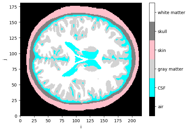
Visualize segmentation masks
[15]:
collapsed_mask = head_ijk.segmentation_masks.sum("segmentation_type")

cmap = ListedColormap(["black", "cyan", "lightgray", "pink", "gray", "white"])
p.pcolormesh(collapsed_mask[:,:, collapsed_mask.sizes["k"]//2], cmap=cmap, vmin=-0.5, vmax=5.5)
cb = p.colorbar()
cb.set_ticks([0,1,2,3,4,5])
cb.set_ticklabels(["air", "CSF", "gray matter", "skin", "skull", "white matter"])
p.xlabel("i")
p.ylabel("j");
Landmarks are stored as LabeledPoints.
[16]:
head_ijk.landmarks
[16]:
<xarray.DataArray (label: 73, ijk: 3)> Size: 2kB
[] 90.0 7.435 48.92 3.924 106.0 24.01 ... 127.4 25.63 109.0 139.8 26.66 93.47
Coordinates:
  * label    (label) <U3 876B 'Iz' 'LPA' 'RPA' 'Nz' ... 'PO1' 'PO2' 'PO4' 'PO6'
    type     (label) object 584B PointType.LANDMARK ... PointType.LANDMARK
Dimensions without coordinates: ijkThe brain and scalp surfaces are represented by triangulated meshes, which are represented by instances of cedalion.dataclasses.TrimeshSurface.
[17]:
head_ijk.brain
[17]:
TrimeshSurface(faces: 49992 vertices: 25000 crs: ijk units: dimensionless vertex_coords: ['fsaverage_vertex', 'parcel', 'mni152_r', 'mni152_a', 'mni152_s'])
[18]:
head_ijk.scalp
[18]:
TrimeshSurface(faces: 20096 vertices: 10050 crs: ijk units: dimensionless vertex_coords: [])
The attribute .crs indicates that the head model and all its components is in voxel space.
[19]:
head_ijk.crs
[19]:
'ijk'
Transformations
The affine transformations between different coordinate reference systems are represented as 4x4 matrices which Cedalion also stores in DataArrays.
The dimension names are chosen such that applying the transformation through matrix multiplication transforms LabeledPoints from one CRS to the other.
The transformation matrix to translate from voxel to scanner space is available as:
[20]:
head_ijk.t_ijk2ras
[20]:
<xarray.DataArray (mni: 4, ijk: 4)> Size: 128B
[mm] 1.0 0.0 0.0 -90.0 0.0 1.0 0.0 -126.0 0.0 0.0 1.0 -72.0 0.0 0.0 0.0 1.0
Dimensions without coordinates: mni, ijk
And the inverse transformation matrix to translate from scanner to voxel space is available as:
[21]:
head_ijk.t_ras2ijk
[21]:
<xarray.DataArray (ijk: 4, mni: 4)> Size: 128B
[1/mm] 1.0 -1.733e-14 -6.085e-15 90.0 ... 3.253e-16 -1.87e-16 -6.487e-17 1.0
Dimensions without coordinates: ijk, mni
The head model provides the function .apply_transform to change the coordinate systems for all components:
[22]:
head_ras = head_ijk.apply_transform(head_ijk.t_ijk2ras)
display(head_ras)
TwoSurfaceHeadModel(
  crs: mni
  tissue_types: csf, gm, scalp, skull, wm
  brain faces: 49992 vertices: 25000 units: millimeter
  scalp faces: 20096 vertices: 10050 units: millimeter
  landmarks: 73
)
Scaling head models or registering optode positions
cedalion has functionality to scale the head model to given head sizes or probe geometries
alternatively, the probe geometry can be scaled to match the head size, changing channel distances in doing so
the scaling affects how large a head model is in scanner space. the result of the scaling is represented in the trafos that connect voxel and scanner space
[23]:
def compare_trafos(t_orig, t_scaled):
    """Compare the length of a unit vector after applying the transform."""
    t_orig = t_orig.pint.dequantify().values
    t_scaled = t_scaled.pint.dequantify().values

    for i, dim in enumerate("xyz"):
        unit_vector = np.zeros(4)
        unit_vector[i] = 1.0
        n1 = np.linalg.norm(t_orig @ unit_vector)
        n2 = np.linalg.norm(t_scaled @ unit_vector)

        print(
            f"After scaling, a unit vector along the {dim}-axis is {n2 / n1 * 100.0:.1f}% "
            "of the original length."
        )
Scale head model using geodesic distances
Transform the head model to the subject’s head size as defined by three measurements:
the head circumference
the distance from Nz through Cz to Iz
the distance from LPA through Cz to RPA
These distances define a ellipsoidal scalp surface to which the head model is fit.
The resulting head will be in CRS=’ellipsoid’.
[24]:
head_scaled = head_ijk.scale_to_headsize(
    circumference=51*units.cm,
    nz_cz_iz=33*units.cm,
    lpa_cz_rpa=33*units.cm
)
display(head_scaled)
TwoSurfaceHeadModel(
  crs: ellipsoid
  tissue_types: csf, gm, scalp, skull, wm
  brain faces: 49992 vertices: 25000 units: millimeter
  scalp faces: 20096 vertices: 10050 units: millimeter
  landmarks: 73
)
Visualize original (green) and scaled (red) scalp surfaces and landmarks.
[25]:
plt = pv.Plotter()
vbx.plot_surface(plt, head_ras.scalp, color="#4fce64", opacity=.1)
vbx.plot_labeled_points(plt, head_ras.landmarks, color="g")
vbx.plot_surface(plt, head_scaled.scalp, color="#ce5c4f")
vbx.plot_labeled_points(plt, head_scaled.landmarks, color="r")
plt.show()
[26]:
compare_trafos(head_ijk.t_ijk2ras, head_scaled.t_ijk2ras)
After scaling, a unit vector along the x-axis is 89.8% of the original length.
After scaling, a unit vector along the y-axis is 76.4% of the original length.
After scaling, a unit vector along the z-axis is 87.3% of the original length.
Scale head model using digitized landmark positions
Transform the head model to the subject’s head size by fitting landmarks of the head model to digitized landmarks.
The resulting head will be in the same CRS as the digitized landmarks. This also affects axis orientations.
[27]:
# Construct LabeledPoints with landmark positions.
# Use the digitized landmarks from 41_photogrammetric_optode_coregistration.ipynb
geo3d = cdc.build_labeled_points(
    [
        [14.00420712, -7.84856869, 449.77840004],
        [99.09920059, 29.72154755, 620.73876117],
        [161.63815139, -48.49738938, 494.91210993],
        [82.8771277, 79.79500128, 498.3338802],
        [15.17214095, -60.56186128, 563.29621021],
    ],
    crs="digitized",
    labels=["Nz", "Iz", "Cz", "LPA", "RPA"],
    types = [cdc.PointType.LANDMARK] * 5,
    units="mm"
)

# shift the center of the landmarks to plot original and
# scaled versions next to each other
geo3d = geo3d - geo3d.mean("label") + (0,200,0)*cedalion.units.mm

head_scaled = head_ijk.scale_to_landmarks(geo3d)
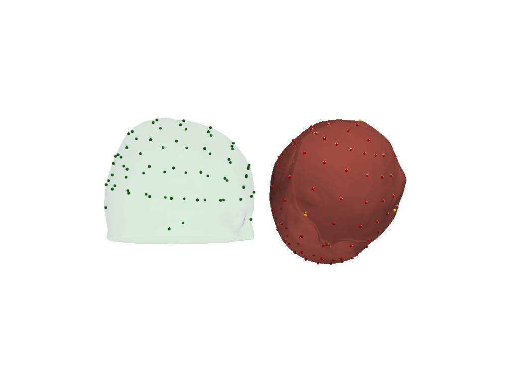
Visualize original (green) and scaled (red) scalp surfaces and landmarks.
The digitized landmarks are plotted in yellow.
[28]:
plt = pv.Plotter()
vbx.plot_surface(plt, head_ras.scalp, color="#4fce64", opacity=.1)
vbx.plot_labeled_points(plt, head_ras.landmarks, color="g")
vbx.plot_surface(plt, head_scaled.scalp, color="#ce5c4f", opacity=.8)
vbx.plot_labeled_points(plt, head_scaled.landmarks, color="r")
vbx.plot_labeled_points(plt, geo3d, color="y", )
vbx.camera_at_cog(plt, head_scaled.scalp, (600,0,0), fit_scene=True)
plt.show()
[29]:
compare_trafos(head_ijk.t_ijk2ras, head_scaled.t_ijk2ras)
After scaling, a unit vector along the x-axis is 98.2% of the original length.
After scaling, a unit vector along the y-axis is 95.9% of the original length.
After scaling, a unit vector along the z-axis is 93.0% of the original length.
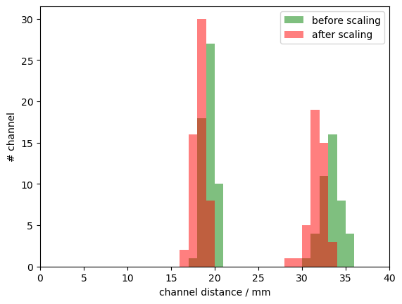
Scale digitized optode positions to head model
Without changing the head model size, transform the optode positions to fit the head model’s landmarks.
The function first aligns the landmarks via an unconstrained affine transformation, then uses spring relaxation to conform the montage to the scalp surface with minimal distortion of channel distances. To derive the unconstrained transformation the digitized coordinates and head model landmarks must contain at least the positions of “Nz”, “Iz”, “Cz”, “LPA”, “RPA”.
If fewer landmarks are available align_and_relax_to_scalp can be called with initial_align_mode='trans_rot_isoscale, which restricts the affine to translations, rotations and isotropic scaling, which have fewer degrees of freedom.
[30]:
geo3d_snapped_ras, alignment_details = head_ras.align_and_relax_to_scalp(rec.geo3d, rec["amp"])
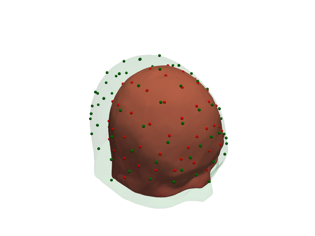
The transformed digitized optode and landmark positions are plotted in red (sources), blue (detectors) and green (landmarks).
The fiducial landmarks of the head model are plotted in yellow.
[31]:
plt = pv.Plotter()
vbx.plot_surface(plt, head_ras.scalp, color="#4fce64", opacity=.1)
vbx.plot_labeled_points(plt, geo3d_snapped_ras)
vbx.plot_labeled_points(
    plt, head_ras.landmarks.sel(label=["Nz", "Iz", "Cz", "LPA", "RPA"]), color="y"
)
plt.show()
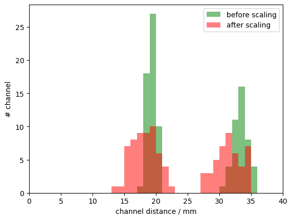
[32]:
bins = np.arange(0, 40.5, 1)
p.hist(cedalion.nirs.channel_distances(rec["amp"], rec.geo3d), bins, label="before scaling", fc="g", alpha=.5)
p.hist(cedalion.nirs.channel_distances(rec["amp"], geo3d_snapped_ras), bins, label="after scaling", fc="r", alpha=.5);
p.legend()
p.xlabel("channel distance / mm")
p.ylabel("# channel")
p.xlim(0,40);
Simulate light propagation in tissue
cedalion.dot.ForwardModel is a wrapper around pmcx and NIRFASTER. It transforms the data in the head model to the input format expected by these photon propagators and offers functionality to calculate the sensitivity matrix.
The forward model operates in voxel space, so we transform the aligned optodes into this CRS.
[33]:
geo3d_snapped_ijk = geo3d_snapped_ras.points.apply_transform(head_ijk.t_ras2ijk)
[34]:
fwm = cedalion.dot.ForwardModel(head_ijk, geo3d_snapped_ijk, meas_list)
Run the simulation
The compute_fluence_mcx and compute_fluence_nirfaster methods simulate a light source at each optode position and calculate the fluence in each voxel. By setting FORWARD_MODEL, you can choose between the pmcx or NIRFASTer package to perform this simulation.
[35]:
if PRECOMPUTED_SENSITIVITY:
    Adot = cedalion.data.get_precomputed_sensitivity("fingertappingDOT", HEAD_MODEL)
else:
    fluence_fname = working_directory / "fluence.h5"
    sensitivity_fname = working_directory / "sensitivity.h5"

    # calculate fluence into fluence file
    if FORWARD_MODEL == "MCX":
        fwm.compute_fluence_mcx(fluence_fname)
    elif FORWARD_MODEL == "NIRFASTER":
        fwm.compute_fluence_nirfaster(fluence_fname)

    # calculate sensitivity from fluence into sensitivity file
    fwm.compute_sensitivity(fluence_fname, sensitivity_fname)

    # load sensitivity
    Adot = cedalion.io.load_Adot(sensitivity_fname)
The result is a sensitivity matrix for each wavelength that describes how changes in absorption at a given brain vertex affect the optical density in a given channel.
[36]:
Adot
[36]:
<xarray.DataArray (channel: 100, vertex: 35050, wavelength: 2)> Size: 28MB
3.656e-17 3.656e-17 1.758e-18 1.758e-18 ... 8.413e-17 2.986e-15 2.986e-15
Coordinates:
    parcel      (vertex) object 280kB 'VisCent_ExStr_8_LH' ... 'scalp'
    is_brain    (vertex) bool 35kB True True True True ... False False False
  * channel     (channel) object 800B 'S1D1' 'S1D2' 'S1D4' ... 'S14D31' 'S14D32'
    source      (channel) object 800B 'S1' 'S1' 'S1' 'S1' ... 'S14' 'S14' 'S14'
    detector    (channel) object 800B 'D1' 'D2' 'D4' 'D5' ... 'D29' 'D31' 'D32'
  * wavelength  (wavelength) float64 16B 760.0 850.0
Dimensions without coordinates: vertex
Attributes: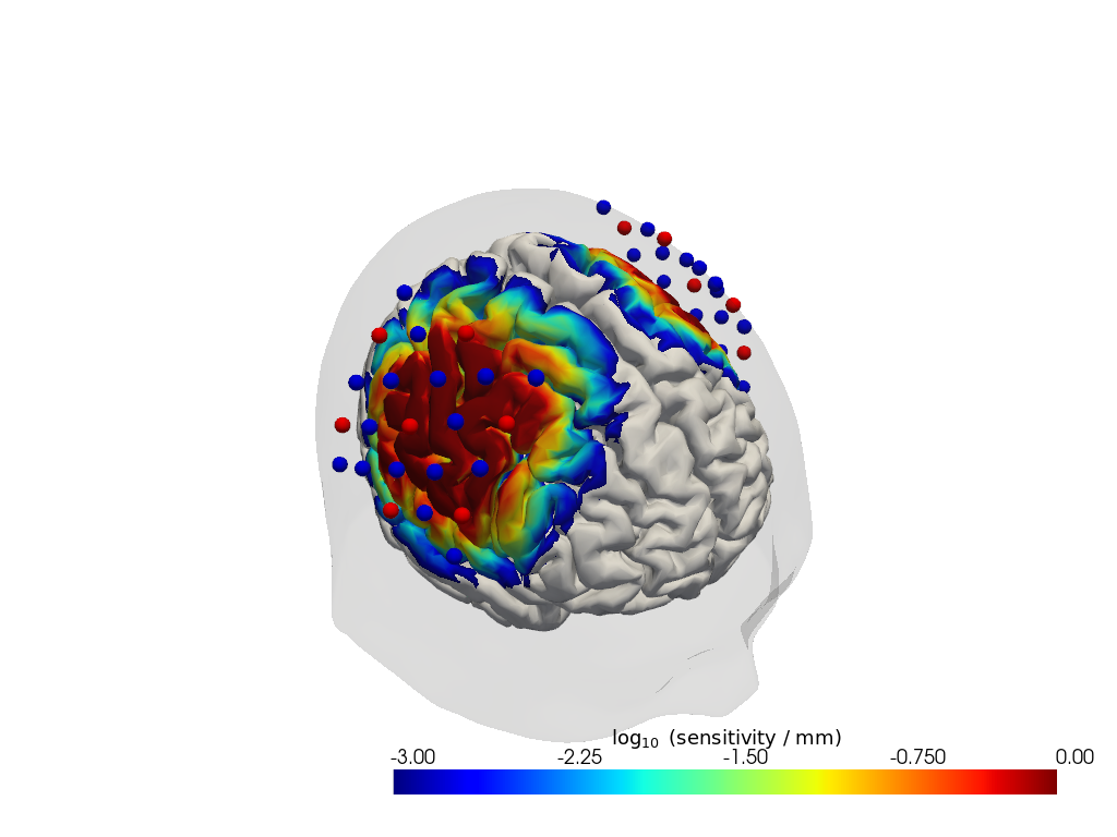
units: mmVisualize the sensitivity
[37]:
# select only a subset of labeled points to plot
# Here we select sources and detectors via their labelsthat start with S or D
geo3d_plot_ijk = geo3d_snapped_ijk.sel(
    label=geo3d_snapped_ijk.label.str.contains("S|D")
)

plotter = cedalion.vis.anatomy.sensitivity_matrix.Main(
    sensitivity=Adot,
    brain_surface=head_ijk.brain,
    head_surface=head_ijk.scalp,
    labeled_points= geo3d_plot_ijk,
)
plotter.plot(high_th=0, low_th=-3)
plotter.plt.show()
References
[38]:
cedalion.bib.dump_to_notebook()
Methods used
| [1] | Tucker2022 | cedalion.io.snirf.read_snirf | Stephen Tucker, Jay Dubb, Sreekanth Kura, Alexander von Lühmann, Robert Franke, Jörn M. Horschig, Samuel Powell, Robert Oostenveld, Michael Lührs, Édouard Delaire, Zahra M. Aghajan, Hanseok Yun, Meryem A. Yücel, Qianqian Fang, Theodore J. Huppert, Blaise deB. Frederick, Luca Pollonini, David A. Boas, and Robert Luke. Introduction to the shared near infrared spectroscopy format. Neurophotonics, 10(1):013507, 2022. doi:10.1117/1.NPh.10.1.013507. |
| [2] | Holmes1998 | cedalion.data.get_colin27_headmodel_files | Colin J. Holmes, Rick Hoge, Louis Collins, Roger Woods, Arthur W. Toga, and Alan C. Evans. Enhancement of mr images using registration for signal averaging. Journal of Computer Assisted Tomography, 22(2):324–333, March 1998. doi:10.1097/00004728-199803000-00032. |
| [3] | Fischl2012 | cedalion.data.get_colin27_headmodel_files | Bruce Fischl. FreeSurfer. NeuroImage, 62(2):774–781, 2012. doi:10.1016/j.neuroimage.2012.01.021. |
| [4] | Schaefer2018 | cedalion.data.get_colin27_headmodel_files | Alexander Schaefer, Ru Kong, Evan M Gordon, Timothy O Laumann, Xi-Nian Zuo, Avram J Holmes, Simon B Eickhoff, and BT Thomas Yeo. Local-global parcellation of the human cerebral cortex from intrinsic functional connectivity mri. Cerebral cortex, 28(9):3095–3114, 2018. doi:10.1093/cercor/bhx179. |
| [5] | Aasted2015 | cedalion.dot.head_model.TwoSurfaceHeadModel.align_and_relax_to_scalp | Christopher M. Aasted, Meryem A. Yücel, Robert J. Cooper, Jay Dubb, Daisuke Tsuzuki, Lino Becerra, Martin P. Petkov, David Borsook, Ippeita Dan, and David A. Boas. Anatomical guidance for functional near-infrared spectroscopy: AtlasViewer tutorial. Neurophotonics, 2(2):020801, 2015. doi:10.1117/1.NPh.2.2.020801. |
| [6] | Fang2009 | cedalion.data.get_precomputed_sensitivity | Qianqian Fang and David A Boas. Monte carlo simulation of photon migration in 3d turbid media accelerated by graphics processing units. Optics express, 17(22):20178–20190, 2009. doi:10.1364/OE.17.020178. |
| [7] | Yu2018 | cedalion.data.get_precomputed_sensitivity | Leiming Yu, Fanny Nina-Paravecino, David Kaeli, and Qianqian Fang. Scalable and massively parallel monte carlo photon transport simulations for heterogeneous computing platforms. Journal of biomedical optics, 23(1):010504–010504, 2018. doi:10.1117/1.JBO.23.1.010504. |
| [8] | Yan2020 | cedalion.data.get_precomputed_sensitivity | Shijie Yan and Qianqian Fang. Hybrid mesh and voxel based monte carlo algorithm for accurate and efficient photon transport modeling in complex bio-tissues. Biomedical Optics Express, 11(11):6262–6270, 2020. doi:10.1364/BOE.409468. |
Next: 2 — Photogrammetry — registering optode positions from a photogrammetric scalp scan to the head model.