Image Reconstruction

# This cells setups the environment when executed in Google Colab.
try:
    import google.colab
    !curl -s https://raw.githubusercontent.com/ibs-lab/cedalion/dev/scripts/colab_setup.py -o colab_setup.py
    # Select branch with --branch "branch name" (default is "dev")
    %run colab_setup.py
except ImportError:
    pass

Notebook configuration

Decide for an example dataset with a sparse probe or a high-density probe for DOT. The notebook will load example data accordingly.

Also specify, if precomputed results of the photon propagation should be used and if the 3D visualizations should be interactive.

# choose between two datasets
DATASET = "fingertappingDOT" # high-density montage
#DATASET = "fingertapping"   # sparse montage

# choose a head model
HEAD_MODEL = "colin27"
# HEAD_MODEL = "icbm152"

# choose between the monte
FORWARD_MODEL = "MCX" # photon monte carlo
#FORWARD_MODEL = "NIRFASTER" # finite element method - NOTE, you must have NIRFASTer installed via runnning <$ bash install_nirfaster.sh CPU # or GPU> from a within your cedalion root directory.

# set this flag to False to actual compute the forward model results
PRECOMPUTED_FLUENCE = True

# set this flag to True to enable interactive 3D plots
INTERACTIVE_PLOTS = False

import pyvista as pv

if INTERACTIVE_PLOTS:
    pv.set_jupyter_backend('server')
else:
    pv.set_jupyter_backend('static')

import time
from pathlib import Path
from tempfile import TemporaryDirectory

import matplotlib.pyplot as p
import numpy as np
import xarray as xr
from IPython.display import Image

import cedalion
import cedalion.data
import cedalion.dataclasses as cdc
import cedalion.dot as dot
#import cedalion.dot.tissue_properties
#import cedalion.geometry.registration
#import cedalion.geometry.segmentation
#import cedalion.io
import cedalion.sigproc.motion_correct as motion_correct
import cedalion.vis.anatomy
import cedalion.vis.anatomy.sensitivity_matrix
import cedalion.vis.blocks as vbx
import cedalion.xrutils as xrutils
from cedalion import units
from cedalion.io.forward_model import FluenceFile, load_Adot

xrutils.unit_stripping_is_error()


xr.set_options(display_expand_data=False);

# helper function to display gifs in rendered notbooks
def display_image(fname : str):
    display(Image(data=open(fname,'rb').read(), format='png'))

Working Directory

In this notebook the output of the fluence and sensitivity calculations are stored in a temporary directory. This will be deleted when the notebook ends.

temporary_directory = TemporaryDirectory()
tmp_dir_path = Path(temporary_directory.name)

Load a finger-tapping dataset

For this demo we load an example finger-tapping recording through either cedalion.data.get_fingertapping or cedalion.data.get_fingertappingDOT.

The snirf files of these datasets contains a single NIRS element with one block of raw amplitude data.

if DATASET == "fingertappingDOT":
    rec = cedalion.data.get_fingertappingDOT()
elif DATASET == "fingertapping":
    rec = cedalion.data.get_fingertapping()
else:
    raise ValueError("unknown dataset")

The location of the probes is obtained from the snirf metadata (i.e. /nirs0/probe/)

Note that units (‘m’) are adopted and the coordinate system is named ‘digitized’.

geo3d_meas = rec.geo3d
display(geo3d_meas)

<xarray.DataArray (label: 346, digitized: 3)> Size: 8kB
[mm] -77.82 15.68 23.17 -61.91 21.23 56.49 ... 14.23 -38.28 81.95 -0.678 -37.03
Coordinates:
    type     (label) object 3kB PointType.SOURCE ... PointType.LANDMARK
  * label    (label) <U6 8kB 'S1' 'S2' 'S3' 'S4' ... 'FFT10h' 'FT10h' 'FTT10h'
Dimensions without coordinates: digitized

xarray.DataArray

• label: 346
• digitized: 3

• [mm] -77.82 15.68 23.17 -61.91 21.23 ... -38.28 81.95 -0.678 -37.03

  Magnitude	[[-77.817871 15.680613999999998 23.172269999999997] [-61.906841 21.227732000000003 56.492802] [-85.37146 -16.079958 8.900885] ... [77.521 28.883 -39.113] [80.59 14.229 -38.278] [81.95 -0.678 -37.027]]
  Units	millimeter

• Coordinates: (2)
  • type
    (label)
    object
    PointType.SOURCE ... PointType.L...

    array([<PointType.SOURCE: 1>, <PointType.SOURCE: 1>, <PointType.SOURCE: 1>,
           ..., <PointType.LANDMARK: 3>, <PointType.LANDMARK: 3>,
           <PointType.LANDMARK: 3>], shape=(346,), dtype=object)

  • label
    (label)
    <U6
    'S1' 'S2' 'S3' ... 'FT10h' 'FTT10h'

    array(['S1', 'S2', 'S3', ..., 'FFT10h', 'FT10h', 'FTT10h'],
          shape=(346,), dtype='<U6')

• Indexes: (1)
  • label
    PandasIndex

    PandasIndex(Index(['S1', 'S2', 'S3', 'S4', 'S5', 'S6', 'S7', 'S8', 'S9', 'S10',
           ...
           'POO10h', 'PO10h', 'PPO10h', 'P10h', 'TPP10h', 'AFF10h', 'F10h',
           'FFT10h', 'FT10h', 'FTT10h'],
          dtype='object', name='label', length=346))

• Attributes: (0)

# visualize the montage
cedalion.vis.anatomy.plot_montage3D(rec["amp"], geo3d_meas)

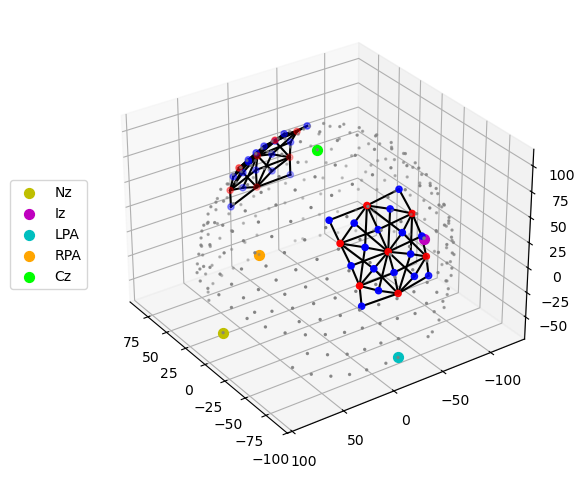
The measurement list is a pandas.DataFrame that describes which source-detector pairs form channels.

meas_list = rec._measurement_lists["amp"]
display(meas_list.head(5))

	sourceIndex	detectorIndex	wavelengthIndex	wavelengthActual	wavelengthEmissionActual	dataType	dataUnit	dataTypeLabel	dataTypeIndex	sourcePower	detectorGain	moduleIndex	sourceModuleIndex	detectorModuleIndex	channel	source	detector	wavelength	chromo
0	1	1	1	None	None	1	None	raw-DC	1	None	None	None	None	None	S1D1	S1	D1	760.0	None
1	1	2	1	None	None	1	None	raw-DC	1	None	None	None	None	None	S1D2	S1	D2	760.0	None
2	1	4	1	None	None	1	None	raw-DC	1	None	None	None	None	None	S1D4	S1	D4	760.0	None
3	1	5	1	None	None	1	None	raw-DC	1	None	None	None	None	None	S1D5	S1	D5	760.0	None
4	1	6	1	None	None	1	None	raw-DC	1	None	None	None	None	None	S1D6	S1	D6	760.0	None

Event/stimulus information is also stored in a pandas.DataFrame.

rec.stim

	onset	duration	value	trial_type
0	23.855104	10.0	1.0	1
1	54.132736	10.0	1.0	1
2	84.410368	10.0	1.0	1
3	114.688000	10.0	1.0	1
4	146.112512	10.0	1.0	1
...	...	...	...	...
125	1431.535616	10.0	1.0	5
126	1526.038528	10.0	1.0	5
127	1650.819072	10.0	1.0	5
128	1805.418496	10.0	1.0	5
129	1931.116544	10.0	1.0	5

130 rows × 4 columns

For clarity, events are given more descriptive names:

if DATASET == "fingertappingDOT":
   rec.stim.cd.rename_events( {
        "1": "Control",
        "2": "FTapping/Left",
        "3": "FTapping/Right",
        "4": "BallSqueezing/Left",
        "5": "BallSqueezing/Right"
    } )
elif DATASET == "fingertapping":
    rec.stim.cd.rename_events( {
        "1.0": "Control",
        "2.0": "FTapping/Left",
        "3.0": "FTapping/Right"
    } )

# count number of trials per trial_type
display(
    rec.stim.groupby("trial_type")[["onset"]]
    .count()
    .rename({"onset": "#trials"}, axis=1)
)

	#trials
trial_type
BallSqueezing/Left	17
BallSqueezing/Right	16
Control	65
FTapping/Left	16
FTapping/Right	16

Preprocessing

Perform motion correction, conversion to optical density and bandpass filtering.

rec["od"] = cedalion.nirs.cw.int2od(rec["amp"])
rec["od_tddr"] = motion_correct.tddr(rec["od"])
rec["od_wavelet"] = motion_correct.wavelet(rec["od_tddr"])

# bandpass filter the data
rec["od_freqfiltered"] = rec["od_wavelet"].cd.freq_filter(
    fmin=0.01, fmax=0.5, butter_order=4
)

Calculate block averages in optical density

# segment data into epochs
epochs = rec["od_freqfiltered"].cd.to_epochs(
    rec.stim,  # stimulus dataframe
    ["FTapping/Left", "FTapping/Right"],  # select fingertapping events, discard others
    before=5 * units.s,  # seconds before stimulus
    after=30 * units.s,  # seconds after stimulus
)

# calculate baseline
baseline = epochs.sel(reltime=(epochs.reltime < 0)).mean("reltime")

# subtract baseline
epochs_blcorrected = epochs - baseline

# group trials by trial_type. For each group individually average the epoch dimension
blockaverage = epochs_blcorrected.groupby("trial_type").mean("epoch")

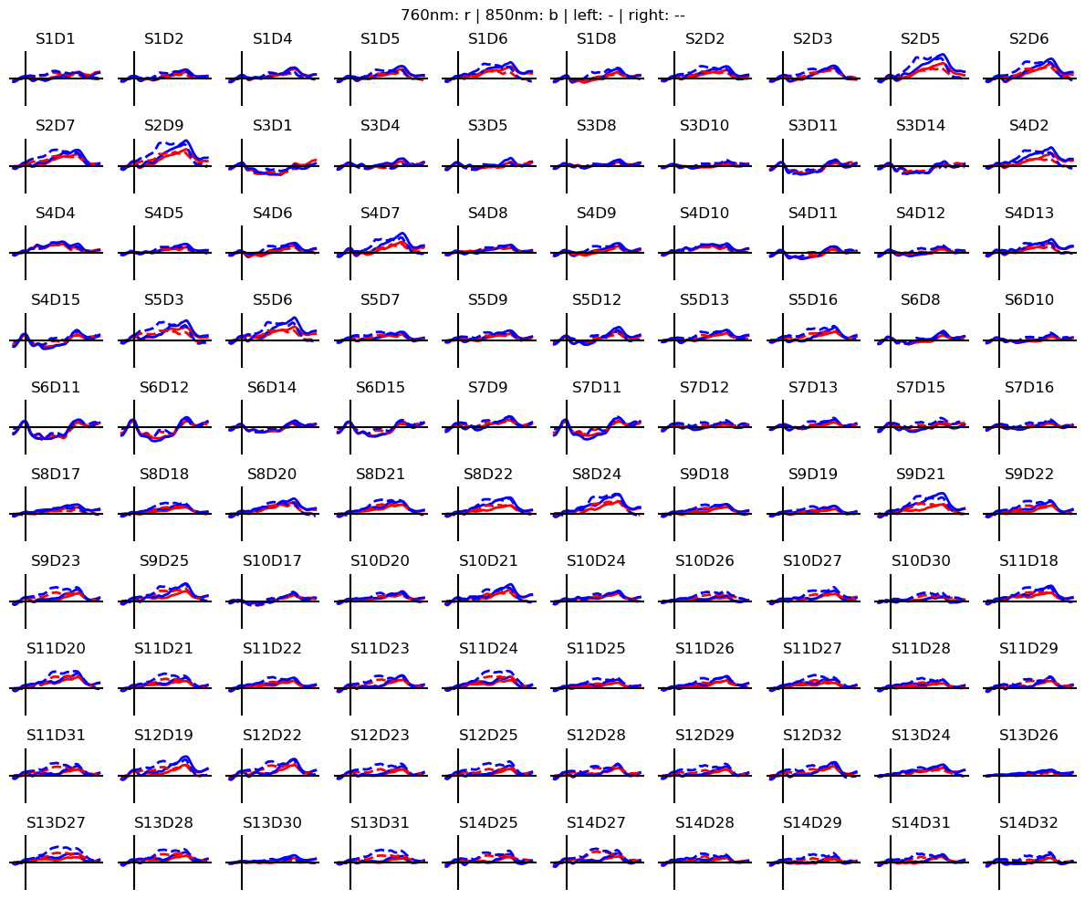
# Plot block averages. Please ignore errors if the plot is too small in the HD case

noPlts2 = int(np.ceil(np.sqrt(len(blockaverage.channel))))
f,ax = p.subplots(noPlts2,noPlts2, figsize=(12,10))
ax = ax.flatten()
for i_ch, ch in enumerate(blockaverage.channel):
    for ls, trial_type in zip(["-", "--"], blockaverage.trial_type):
        ax[i_ch].plot(blockaverage.reltime, blockaverage.sel(wavelength=760, trial_type=trial_type, channel=ch), "r", lw=2, ls=ls)
        ax[i_ch].plot(blockaverage.reltime, blockaverage.sel(wavelength=850, trial_type=trial_type, channel=ch), "b", lw=2, ls=ls)

    ax[i_ch].grid(1)
    ax[i_ch].set_title(ch.values)
    ax[i_ch].set_ylim(-.02, .02)
    ax[i_ch].set_axis_off()
    ax[i_ch].axhline(0, c="k")
    ax[i_ch].axvline(0, c="k")

p.suptitle("760nm: r | 850nm: b | left: - | right: --")
p.tight_layout()

Coordinate systems

Up to now we have geometrical data from three different coordinate reference systems (CRS):

• The optode positions are in one space CRS='digitized' and the coordinates are in meter. In our example the origin is at the head center and y-axis pointing in the superior direction. Other digitization tools can use other units or coordinate systems.

• The segmentation masks are in voxel space (CRS='ijk') in which the voxel edges are aligned with the coordinate axes. Each voxel has unit edge length, i.e. coordinates are dimensionless. Axis-aligned grids are computationally efficient, which is why the photon simulation code (MCX) uses this coordinate system.

• The voxel space (CRS='ijk') is related to scanner space (CRS='ras') in which coordinates have physical units and coordinate axes point to the (r)ight, (a)nterior and s(uperior) directions. The relation between both spaces is given through an affine transformation (e.g. t_ijk2ras). When loading the segmentation masks in Slicer3D this transformation is automatically applied. Hence, the picked landmark coordinates are exported in RAS space.

The scanner space of the standard Colin27 and ICBM152 head models is called CRS='mni'. When loading a subject-specific nifiti file, the file contains a string label for the RAS space. Cedalion uses this string label to name the crs.

To avoid confusion between these different coordinate systems, cedalion tries to be explicit about which CRS a given point cloud or surface is in.

The TwoSurfaceHeadModel

The photon propagation considers the complete MRI scan, in which each voxel is attributed to one tissue type with its respective optical properties. However, the image reconstruction does not intend to reconstruct absorption changes in each voxel. The inverse problem is simplified, by considering only two surfaces (scalp and brain) and reconstruct only absorption changes in voxels close to these surfaces.

The class cedalion.dot.TwoSurfaceHeadModel groups together the segmentation mask, landmark positions and affine transformations as well as the scalp and brain surfaces. The brain surface is calculated by grouping together white and gray matter masks. The scalp surface encloses the whole head.

head_ijk = dot.get_standard_headmodel(HEAD_MODEL)
head_ijk

TwoSurfaceHeadModel(
  crs: ijk
  tissue_types: csf, gm, scalp, skull, wm
  brain faces: 29988 vertices: 15002 units: dimensionless
  scalp faces: 20096 vertices: 10050 units: dimensionless
  landmarks: 73
)

Segmentation masks:

head_ijk.segmentation_masks

<xarray.DataArray (segmentation_type: 5, i: 181, j: 217, k: 181)> Size: 36MB
0 0 0 0 0 0 0 0 0 0 0 0 0 0 0 0 0 0 0 ... 0 0 0 0 0 0 0 0 0 0 0 0 0 0 0 0 0 0 0
Coordinates:
  * segmentation_type  (segmentation_type) <U5 100B 'csf' 'gm' ... 'skull' 'wm'
Dimensions without coordinates: i, j, k

xarray.DataArray

• segmentation_type: 5
• i: 181
• j: 217
• k: 181

• 0 0 0 0 0 0 0 0 0 0 0 0 0 0 0 0 0 ... 0 0 0 0 0 0 0 0 0 0 0 0 0 0 0 0

  array([[[[0, 0, 0, ..., 0, 0, 0],
           [0, 0, 0, ..., 0, 0, 0],
           [0, 0, 0, ..., 0, 0, 0],
           ...,
           [0, 0, 0, ..., 0, 0, 0],
           [0, 0, 0, ..., 0, 0, 0],
           [0, 0, 0, ..., 0, 0, 0]],
  
          [[0, 0, 0, ..., 0, 0, 0],
           [0, 0, 0, ..., 0, 0, 0],
           [0, 0, 0, ..., 0, 0, 0],
           ...,
           [0, 0, 0, ..., 0, 0, 0],
           [0, 0, 0, ..., 0, 0, 0],
           [0, 0, 0, ..., 0, 0, 0]],
  
          [[0, 0, 0, ..., 0, 0, 0],
           [0, 0, 0, ..., 0, 0, 0],
           [0, 0, 0, ..., 0, 0, 0],
           ...,
  ...
           ...,
           [0, 0, 0, ..., 0, 0, 0],
           [0, 0, 0, ..., 0, 0, 0],
           [0, 0, 0, ..., 0, 0, 0]],
  
          [[0, 0, 0, ..., 0, 0, 0],
           [0, 0, 0, ..., 0, 0, 0],
           [0, 0, 0, ..., 0, 0, 0],
           ...,
           [0, 0, 0, ..., 0, 0, 0],
           [0, 0, 0, ..., 0, 0, 0],
           [0, 0, 0, ..., 0, 0, 0]],
  
          [[0, 0, 0, ..., 0, 0, 0],
           [0, 0, 0, ..., 0, 0, 0],
           [0, 0, 0, ..., 0, 0, 0],
           ...,
           [0, 0, 0, ..., 0, 0, 0],
           [0, 0, 0, ..., 0, 0, 0],
           [0, 0, 0, ..., 0, 0, 0]]]], shape=(5, 181, 217, 181), dtype=uint8)

• Coordinates: (1)
  • segmentation_type
    (segmentation_type)
    <U5
    'csf' 'gm' 'scalp' 'skull' 'wm'

    array(['csf', 'gm', 'scalp', 'skull', 'wm'], dtype='<U5')

• Indexes: (1)
  • segmentation_type
    PandasIndex

    PandasIndex(Index(['csf', 'gm', 'scalp', 'skull', 'wm'], dtype='object', name='segmentation_type'))

• Attributes: (0)

Landmarks:

head_ijk.landmarks

<xarray.DataArray (label: 73, ijk: 3)> Size: 2kB
[] 90.0 7.435 48.92 3.924 106.0 24.01 ... 127.4 25.63 109.0 139.8 26.66 93.47
Coordinates:
  * label    (label) <U3 876B 'Iz' 'LPA' 'RPA' 'Nz' ... 'PO1' 'PO2' 'PO4' 'PO6'
    type     (label) object 584B PointType.LANDMARK ... PointType.LANDMARK
Dimensions without coordinates: ijk

xarray.DataArray

• label: 73
• ijk: 3

• [] 90.0 7.435 48.92 3.924 106.0 ... 25.63 109.0 139.8 26.66 93.47

  Magnitude

  [[90.00449999997136 7.4349999999599135 48.9219999999771] [3.923900000023451 106.01030000003283 24.014000000018775] [175.79390000002348 105.99070000003289 23.969000000018802] [89.32080500005482 209.25934700007684 32.59147300004392] [90.93842294426845 116.03494793847557 169.7001348948721] [8.31992218141012 108.51306834604861 60.36205733856532] [175.24822298717078 108.65765488429471 62.69427025514189] [89.69059915337971 213.47141148324624 70.4752402321002] [90.08564815381916 206.60882514786448 108.03477300933892] [90.45067855154238 184.64125761181265 138.73614323220036] [90.74735404491972 153.08353683382467 160.17697836226372] [91.0454332835939 78.81350933305171 170.81291222806453] [90.97156372487827 44.70048763028197 154.71977498752847] [90.69940353126124 24.8690766480575 122.55090831005816] [90.37136656855918 11.588956260808757 86.49950412515159] [60.69490482168986 209.83855643251957 64.21688320737701] [36.063745183876776 194.3548538525447 59.87517725181218] [21.565616907916095 168.0862589916713 58.66819815137465] [11.813265987187819 139.85819435202933 58.68631883144499] [7.877149512179528 80.18668117510077 62.48895699438084] [19.318829371980073 52.88123333883979 67.21776218410916] [36.071546623584055 28.701720374621246 72.89945904229214] [61.4535901560261 14.583940670376293 79.73769655446029] [119.88123436314007 210.2650246048555 65.02685954115795] [146.2214083000308 196.1737267783402 61.176992812809914] [162.69299584704913 170.61168375452314 60.109719508195994] [172.26094733289136 141.4208204942143 60.63732858045386] [174.33583195064733 81.06122411706612 65.07470877470165] [163.51091817228092 52.37349349036484 69.41556881298489] [146.30910717371273 27.964397046968884 74.61909006781498] [120.07501106073948 14.424005035455451 80.65976299729516] [11.56729266576636 111.20990207075816 99.5264769619847] [24.39955584376783 113.71465699427702 135.91514182310328] [53.83342863670708 115.4392691087865 160.9987375402406] [128.48380888554007 115.40968061128765 160.67316286548078] [158.80877782607104 113.75895021322005 136.7456911697093] [173.44633794563174 111.33027724597241 101.50008491406912] [14.960373165805578 144.35331513336558 94.75506964251704] [29.90000027057244 148.5088241946282 127.2994903039669] [56.168156108409775 151.79283682935545 152.0578361455972] [125.84202154631143 152.29273106928053 151.4630931417327] [153.08052269862446 149.5750506862277 127.72034230673675] [170.23245289809876 145.81891565205646 96.26690201681389] [26.177672212912164 173.76073772633612 87.679657477522] [39.879980245515235 179.00703402743414 113.72357303965626] [62.143054570093696 182.94265012880578 132.27258105433688] [119.90002899673357 183.92690090707708 132.60722490894153] [142.02480047761279 180.64562500259464 113.78664040662902] [157.39142787437407 176.0037658798997 88.47607592993509] [45.02411110786035 198.59113440200122 77.08039483909032] [56.665488309099345 202.37925095524844 92.2577149386125] [72.04613988798512 205.3233038782646 103.69072245545583] [109.92722674762682 206.0425332961488 104.53051602881871] [125.19469208596655 203.46988753281823 92.89657016923393] [136.4388228880121 199.90216503198184 77.33104560094722] [13.013301397689219 79.56998280578881 100.62951882056436] [26.296244123636562 79.03739184593594 136.4542386131974] [54.14711148382957 78.7492022569088 162.57949251666048] [128.90147412902638 79.1439641518408 163.62149074743235] [157.56090095711068 79.72426843752518 138.65669438887556] [172.13998273775422 80.39950188819381 103.48589009918604] [24.302016583352028 49.98403974642616 98.67819661031876] [37.56370789212251 47.3636791677267 126.92997889647486] [61.615998781572095 45.484545519937214 146.85368881440064] [122.50785855318719 45.14150171309639 149.1836848429788] [146.2515881595793 46.94627490981749 128.96463918708105] [158.8032124857133 49.538818770260576 100.41882777184898] [42.57802828271425 27.295457379294504 92.1806121768327] [54.45468110426892 26.108645323333732 107.95139546258376] [70.79383449093712 25.15873342880147 120.03750878472157] [110.05884124330703 24.98220241671096 119.43832178938095] [127.44839718973225 25.625637574565104 109.01671619342518] [139.80987741327417 26.660939165583287 93.47475721288436]]

  Units

  dimensionless

• Coordinates: (2)
  • label
    (label)
    <U3
    'Iz' 'LPA' 'RPA' ... 'PO4' 'PO6'

    array(['Iz', 'LPA', 'RPA', 'Nz', 'Cz', 'T7', 'T8', 'Fpz', 'AFz', 'Fz', 'FCz',
           'CPz', 'Pz', 'POz', 'Oz', 'Fp1', 'AF7', 'F7', 'FT7', 'TP7', 'P7', 'PO7',
           'O1', 'Fp2', 'AF8', 'F8', 'FT8', 'TP8', 'P8', 'PO8', 'O2', 'C5', 'C3',
           'C1', 'C2', 'C4', 'C6', 'FC5', 'FC3', 'FC1', 'FC2', 'FC4', 'FC6', 'F5',
           'F3', 'F1', 'F2', 'F4', 'F6', 'AF5', 'AF3', 'AF1', 'AF2', 'AF4', 'AF6',
           'CP5', 'CP3', 'CP1', 'CP2', 'CP4', 'CP6', 'P5', 'P3', 'P1', 'P2', 'P4',
           'P6', 'PO5', 'PO3', 'PO1', 'PO2', 'PO4', 'PO6'], dtype='<U3')

  • type
    (label)
    object
    PointType.LANDMARK ... PointType...

    array([<PointType.LANDMARK: 3>, <PointType.LANDMARK: 3>,
           <PointType.LANDMARK: 3>, <PointType.LANDMARK: 3>,
           <PointType.LANDMARK: 3>, <PointType.LANDMARK: 3>,
           <PointType.LANDMARK: 3>, <PointType.LANDMARK: 3>,
           <PointType.LANDMARK: 3>, <PointType.LANDMARK: 3>,
           <PointType.LANDMARK: 3>, <PointType.LANDMARK: 3>,
           <PointType.LANDMARK: 3>, <PointType.LANDMARK: 3>,
           <PointType.LANDMARK: 3>, <PointType.LANDMARK: 3>,
           <PointType.LANDMARK: 3>, <PointType.LANDMARK: 3>,
           <PointType.LANDMARK: 3>, <PointType.LANDMARK: 3>,
           <PointType.LANDMARK: 3>, <PointType.LANDMARK: 3>,
           <PointType.LANDMARK: 3>, <PointType.LANDMARK: 3>,
           <PointType.LANDMARK: 3>, <PointType.LANDMARK: 3>,
           <PointType.LANDMARK: 3>, <PointType.LANDMARK: 3>,
           <PointType.LANDMARK: 3>, <PointType.LANDMARK: 3>,
           <PointType.LANDMARK: 3>, <PointType.LANDMARK: 3>,
           <PointType.LANDMARK: 3>, <PointType.LANDMARK: 3>,
           <PointType.LANDMARK: 3>, <PointType.LANDMARK: 3>,
           <PointType.LANDMARK: 3>, <PointType.LANDMARK: 3>,
           <PointType.LANDMARK: 3>, <PointType.LANDMARK: 3>,
           <PointType.LANDMARK: 3>, <PointType.LANDMARK: 3>,
           <PointType.LANDMARK: 3>, <PointType.LANDMARK: 3>,
           <PointType.LANDMARK: 3>, <PointType.LANDMARK: 3>,
           <PointType.LANDMARK: 3>, <PointType.LANDMARK: 3>,
           <PointType.LANDMARK: 3>, <PointType.LANDMARK: 3>,
           <PointType.LANDMARK: 3>, <PointType.LANDMARK: 3>,
           <PointType.LANDMARK: 3>, <PointType.LANDMARK: 3>,
           <PointType.LANDMARK: 3>, <PointType.LANDMARK: 3>,
           <PointType.LANDMARK: 3>, <PointType.LANDMARK: 3>,
           <PointType.LANDMARK: 3>, <PointType.LANDMARK: 3>,
           <PointType.LANDMARK: 3>, <PointType.LANDMARK: 3>,
           <PointType.LANDMARK: 3>, <PointType.LANDMARK: 3>,
           <PointType.LANDMARK: 3>, <PointType.LANDMARK: 3>,
           <PointType.LANDMARK: 3>, <PointType.LANDMARK: 3>,
           <PointType.LANDMARK: 3>, <PointType.LANDMARK: 3>,
           <PointType.LANDMARK: 3>, <PointType.LANDMARK: 3>,
           <PointType.LANDMARK: 3>], dtype=object)

• Indexes: (1)
  • label
    PandasIndex

    PandasIndex(Index(['Iz', 'LPA', 'RPA', 'Nz', 'Cz', 'T7', 'T8', 'Fpz', 'AFz', 'Fz', 'FCz',
           'CPz', 'Pz', 'POz', 'Oz', 'Fp1', 'AF7', 'F7', 'FT7', 'TP7', 'P7', 'PO7',
           'O1', 'Fp2', 'AF8', 'F8', 'FT8', 'TP8', 'P8', 'PO8', 'O2', 'C5', 'C3',
           'C1', 'C2', 'C4', 'C6', 'FC5', 'FC3', 'FC1', 'FC2', 'FC4', 'FC6', 'F5',
           'F3', 'F1', 'F2', 'F4', 'F6', 'AF5', 'AF3', 'AF1', 'AF2', 'AF4', 'AF6',
           'CP5', 'CP3', 'CP1', 'CP2', 'CP4', 'CP6', 'P5', 'P3', 'P1', 'P2', 'P4',
           'P6', 'PO5', 'PO3', 'PO1', 'PO2', 'PO4', 'PO6'],
          dtype='object', name='label'))

• Attributes: (0)

Brain surface:

head_ijk.brain

TrimeshSurface(faces: 29988 vertices: 15002 crs: ijk units: dimensionless vertex_coords: ['parcel'])

Scalp Surface:

head_ijk.scalp

TrimeshSurface(faces: 20096 vertices: 10050 crs: ijk units: dimensionless vertex_coords: [])

The loaded head model is in voxel space (CRS='ijk'):

head_ijk.crs

'ijk'

The transformation matrix to translate from voxel to scanner space:

head_ijk.t_ijk2ras

<xarray.DataArray (mni: 4, ijk: 4)> Size: 128B
[mm] 1.0 0.0 0.0 -90.0 0.0 1.0 0.0 -126.0 0.0 0.0 1.0 -72.0 0.0 0.0 0.0 1.0
Dimensions without coordinates: mni, ijk

xarray.DataArray

• mni: 4
• ijk: 4

• [mm] 1.0 0.0 0.0 -90.0 0.0 1.0 0.0 ... 0.0 1.0 -72.0 0.0 0.0 0.0 1.0

  Magnitude	[[1.0 0.0 0.0 -90.0] [0.0 1.0 0.0 -126.0] [0.0 0.0 1.0 -72.0] [0.0 0.0 0.0 1.0]]
  Units	millimeter

• Coordinates: (0)
• Indexes: (0)
• Attributes: (0)

Change from voxel to scanner space. Note the changes in CRS and units.

The function TwoSurfaceHeadmodel.apply_transform transforms all surfaces and landmarks that comprise the head model.

head_ras = head_ijk.apply_transform(head_ijk.t_ijk2ras)
print(f"CRS is now '{head_ras.crs}'")
print("Scalp surface:", head_ras.scalp)
print("Brain surface:", head_ras.brain)
print(f"Landmarks CRS: '{head_ras.landmarks.points.crs}' units: {head_ras.landmarks.pint.units}")
head_ras

CRS is now 'mni'
Scalp surface: TrimeshSurface(faces: 20096 vertices: 10050 crs: mni units: millimeter vertex_coords: [])
Brain surface: TrimeshSurface(faces: 29988 vertices: 15002 crs: mni units: millimeter vertex_coords: ['parcel'])
Landmarks CRS: 'mni' units: millimeter

TwoSurfaceHeadModel(
  crs: mni
  tissue_types: csf, gm, scalp, skull, wm
  brain faces: 29988 vertices: 15002 units: millimeter
  scalp faces: 20096 vertices: 10050 units: millimeter
  landmarks: 73
)

Optode Registration

The optode coordinates from the recording must be aligned with the scalp surface. Currently, cedaĺion offers only a simple registration method, which finds an affine transformation (scaling, rotating, translating) that matches the landmark positions of the head model and their digitized counter parts. Afterwards, optodes are snapped to the nearest vertex on the scalp.

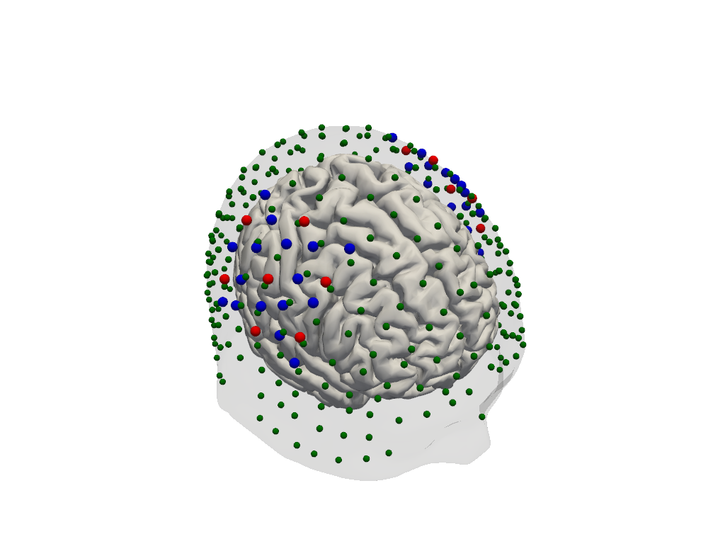
geo3d_snapped_ijk = head_ijk.align_and_snap_to_scalp(geo3d_meas)
display(geo3d_snapped_ijk)

<xarray.DataArray (label: 346, ijk: 3)> Size: 8kB
[] 15.1 140.9 100.2 30.75 144.6 130.6 ... 172.5 137.6 42.28 172.7 126.0 43.07
Coordinates:
    type     (label) object 3kB PointType.SOURCE ... PointType.LANDMARK
  * label    (label) <U6 8kB 'S1' 'S2' 'S3' 'S4' ... 'FFT10h' 'FT10h' 'FTT10h'
Dimensions without coordinates: ijk

xarray.DataArray

• label: 346
• ijk: 3

• [] 15.1 140.9 100.2 30.75 144.6 ... 137.6 42.28 172.7 126.0 43.07

  Magnitude	[[15.104272 140.885747 100.193729] [30.751639 144.623198 130.572037] [9.493661 110.769593 82.930916] ... [169.936666 156.002784 42.818584] [172.538797 137.606965 42.284837] [172.660486 125.957309 43.067074]]
  Units	dimensionless

• Coordinates: (2)
  • type
    (label)
    object
    PointType.SOURCE ... PointType.L...

    array([<PointType.SOURCE: 1>, <PointType.SOURCE: 1>, <PointType.SOURCE: 1>,
           ..., <PointType.LANDMARK: 3>, <PointType.LANDMARK: 3>,
           <PointType.LANDMARK: 3>], shape=(346,), dtype=object)

  • label
    (label)
    <U6
    'S1' 'S2' 'S3' ... 'FT10h' 'FTT10h'

    array(['S1', 'S2', 'S3', ..., 'FFT10h', 'FT10h', 'FTT10h'],
          shape=(346,), dtype='<U6')

• Indexes: (1)
  • label
    PandasIndex

    PandasIndex(Index(['S1', 'S2', 'S3', 'S4', 'S5', 'S6', 'S7', 'S8', 'S9', 'S10',
           ...
           'POO10h', 'PO10h', 'PPO10h', 'P10h', 'TPP10h', 'AFF10h', 'F10h',
           'FFT10h', 'FT10h', 'FTT10h'],
          dtype='object', name='label', length=346))

• Attributes: (0)

plt = pv.Plotter()
vbx.plot_surface(plt, head_ijk.brain, color="w")
vbx.plot_surface(plt, head_ijk.scalp, opacity=.1)
vbx.plot_labeled_points(plt, geo3d_snapped_ijk)
plt.show()

Simulate light propagation in tissue

cedalion.dot.ForwardModel wraps the photon propagation codes pmcx and nirfaster.

Using the data in the head model it prepares the inputs for either pmcx or NIRFASTer and offers functionality to calculate the sensitivty matrix.

fwm = dot.ForwardModel(head_ijk, geo3d_snapped_ijk, meas_list)

Run the simulation

The compute_fluence_mcx and compute_fluence_nirfaster methods simulate a light source at each optode position and calculate the fluence in each voxel. By setting RUN_PACKAGE, you can choose between the pmcx or NIRFASTer package to perform this simulation.

PLEASE NOTE: if you use precomputed data (download the example data) be aware that the file is quite big (~2GB).

if PRECOMPUTED_FLUENCE:
    if FORWARD_MODEL == "MCX":
        fluence_fname = cedalion.data.get_precomputed_fluence(DATASET, HEAD_MODEL)
    elif FORWARD_MODEL == "NIRFASTER":
        raise NotImplementedError(
            "Currently there are no precomputed NIRFASTER results available"
        )
else:
    fluence_fname = tmp_dir_path / "fluence.h5"

    if FORWARD_MODEL == "MCX":
        fwm.compute_fluence_mcx(fluence_fname)
    elif FORWARD_MODEL == "NIRFASTER":
        fwm.compute_fluence_nirfaster(fluence_fname)

The photon simulation yields the fluence in each voxel for each wavelength. This is stored in two data structures:

• fluence_all is an array with dimensions: (‘label’, ‘wavelength’, ‘i’, ‘j’, ‘k’),

  i.e. for each optode and wavelength it stores the 3D image of the computed fluence in each voxel

• fluence_at_optodes is an array with dimensions: (‘optode1’, ‘optode2’, ‘wavelength’).

  It contains the fluence directly at the position of the optodes which is needed for normalization purposes.

Both arrays are stored on disk in a hdf5 file at fluence_fname. The class cedalion.io.forward_model.FluenceFile provides functions to query data from the file.

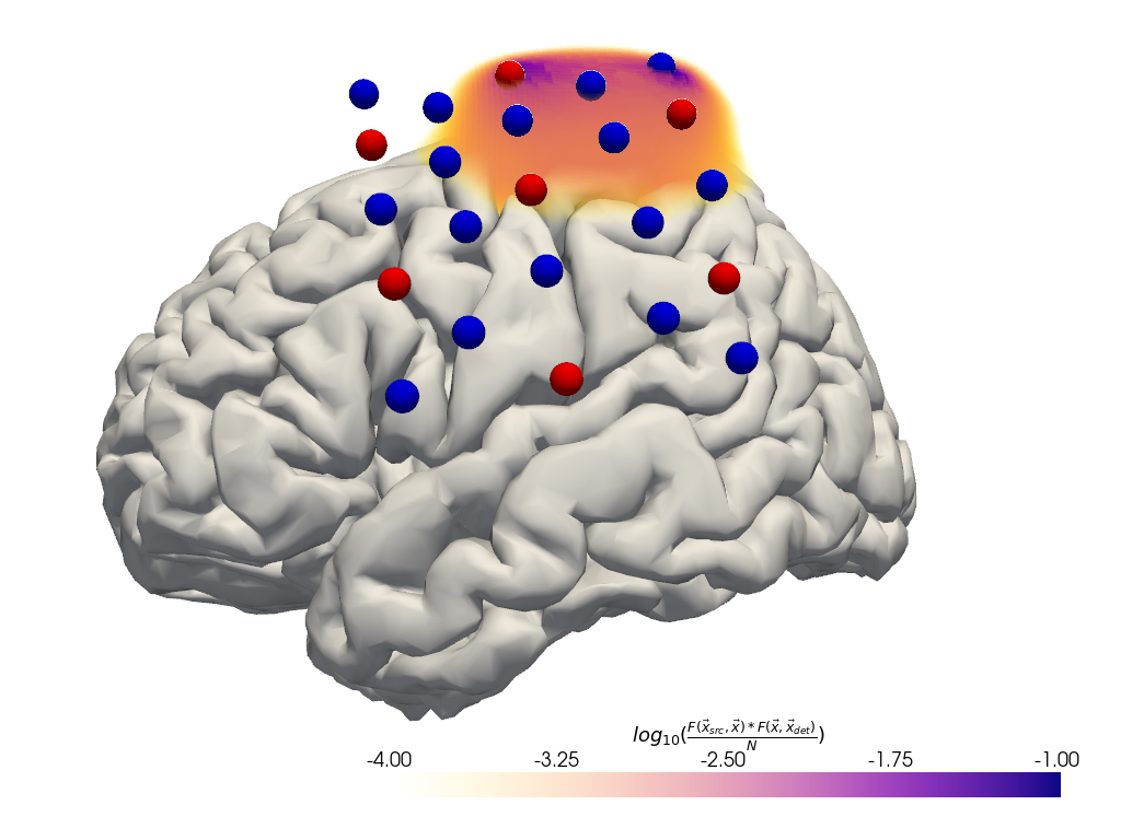
Plot fluence

To illustrate the tissue probed by light travelling from a source to the detector two fluence profiles need to be multiplied.

# for plotting remove the landmarks from geo3d
geo3d_plot = geo3d_snapped_ijk[geo3d_snapped_ijk.type != cdc.PointType.LANDMARK]

#time.sleep(1)

plt = pv.Plotter()

if DATASET == "fingertappingDOT":
    src, det, wl = "S5", "D16", 760
elif DATASET == "fingertapping":
    src, det, wl = "S2", "D3", 760
else:
    raise ValueError("unknown dataset")

# fluence_file.get_fluence returns a 3D numpy array with the fluence
# for a specified source and wavelength.
with FluenceFile(fluence_fname) as fluence_file:
    f = fluence_file.get_fluence(src, wl) * fluence_file.get_fluence(det, wl)
    fao = fluence_file.get_fluence_at_optodes()
    f /= 0.5 * (fao.loc[src, det, wl].values + fao.loc[det, src, wl].values)


f = np.log10(np.clip(f, min=f[f > 0].min()))
vf = pv.wrap(f)

print(f.min(), f.max())

plt.add_volume(
    vf,
    log_scale=False,
    cmap="plasma_r",
    clim=(-4, -1),
    scalar_bar_args={
        "title": r"$log_{10}("
        r"\frac{F(\vec{x}_{src},\vec{x}) * F(\vec{x}, \vec{x}_{det})}{N}"
        ")$"
    },
)
vbx.plot_surface(plt, head_ijk.brain, color="w")
vbx.plot_labeled_points(plt, geo3d_plot, show_labels=False)
vbx.camera_at_cog(plt, head_ijk.brain, rpos=[-350, 50, -50], fp_offset=[0, -10, 0])
plt.show()

-36.334373 0.3564576

Calculate the sensitivity matrices

The forward model’s function compute_sensitivity calculates the sensitivity matrix from the fluence file and saves the result in a new file.

if PRECOMPUTED_FLUENCE:
    Adot = cedalion.data.get_precomputed_sensitivity(DATASET, HEAD_MODEL)
else:
    sensitivity_fname = tmp_dir_path / "sensitivity.h5"
    fwm.compute_sensitivity(fluence_fname, sensitivity_fname)
    Adot = load_Adot(sensitivity_fname)

The sensitivity matrix describes how an absorption change at a given surface vertex changes the optical density in a given channel and wavelength.

The coordinate is_brain holds a mask to distinguish brain and scalp voxels.

Adot

<xarray.DataArray (channel: 100, vertex: 25052, wavelength: 2)> Size: 40MB
1.212e-17 1.212e-17 3.962e-20 3.962e-20 ... 1.96e-18 3.815e-16 3.815e-16
Coordinates:
    parcel      (vertex) object 200kB 'VisCent_ExStr_8_LH' ... 'scalp'
    is_brain    (vertex) bool 25kB True True True True ... False False False
  * channel     (channel) object 800B 'S1D1' 'S1D2' 'S1D4' ... 'S14D31' 'S14D32'
    source      (channel) object 800B 'S1' 'S1' 'S1' 'S1' ... 'S14' 'S14' 'S14'
    detector    (channel) object 800B 'D1' 'D2' 'D4' 'D5' ... 'D29' 'D31' 'D32'
  * wavelength  (wavelength) float64 16B 760.0 850.0
Dimensions without coordinates: vertex
Attributes: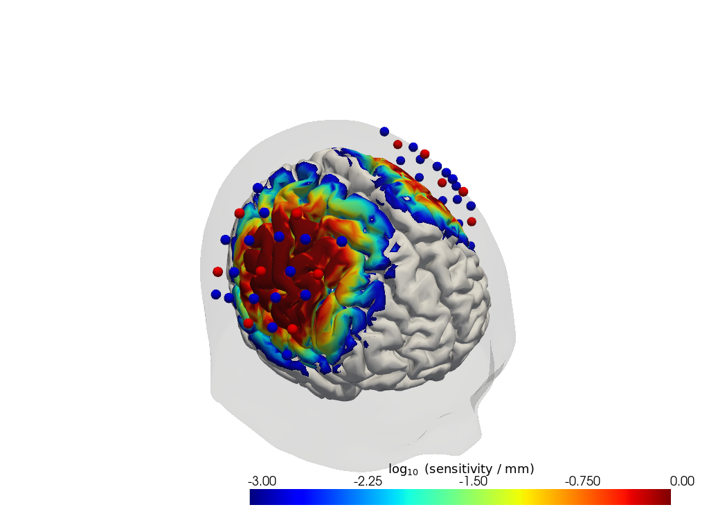
    units:    mm

xarray.DataArray

• channel: 100
• vertex: 25052
• wavelength: 2

• 1.212e-17 1.212e-17 3.962e-20 ... 1.96e-18 3.815e-16 3.815e-16

  array([[[1.21179827e-17, 1.21179827e-17],
          [3.96194809e-20, 3.96194809e-20],
          [4.10971853e-19, 4.10971853e-19],
          ...,
          [3.50555240e-12, 3.50555240e-12],
          [5.26119937e-13, 5.26119937e-13],
          [8.08679933e-13, 8.08679933e-13]],
  
         [[7.61680927e-18, 7.61680927e-18],
          [1.23019221e-18, 1.23019221e-18],
          [1.67531031e-19, 1.67531031e-19],
          ...,
          [2.33481439e-12, 2.33481439e-12],
          [4.92126651e-13, 4.92126651e-13],
          [1.07023130e-12, 1.07023130e-12]],
  
         [[5.52717640e-17, 5.52717640e-17],
          [1.78701021e-18, 1.78701021e-18],
          [6.99671883e-18, 6.99671883e-18],
          ...,
  ...
          ...,
          [5.98963847e-19, 5.98963847e-19],
          [6.62891414e-18, 6.62891414e-18],
          [1.28914788e-15, 1.28914788e-15]],
  
         [[3.15260006e-12, 3.15260006e-12],
          [8.79590880e-12, 8.79590880e-12],
          [1.06539458e-11, 1.06539458e-11],
          ...,
          [3.80802873e-19, 3.80802873e-19],
          [1.03147281e-16, 1.03147281e-16],
          [2.13242570e-16, 2.13242570e-16]],
  
         [[2.51903559e-12, 2.51903559e-12],
          [6.00967488e-12, 6.00967488e-12],
          [1.87582313e-12, 1.87582313e-12],
          ...,
          [2.80353969e-20, 2.80353969e-20],
          [1.96006079e-18, 1.96006079e-18],
          [3.81463022e-16, 3.81463022e-16]]], shape=(100, 25052, 2))

• Coordinates: (6)
  • parcel
    (vertex)
    object
    'VisCent_ExStr_8_LH' ... 'scalp'

    array(['VisCent_ExStr_8_LH', 'VisCent_ExStr_8_LH', 'VisCent_Striate_2_LH',
           ..., 'scalp', 'scalp', 'scalp'], shape=(25052,), dtype=object)

  • is_brain
    (vertex)
    bool
    True True True ... False False

    array([ True,  True,  True, ..., False, False, False], shape=(25052,))

  • channel
    (channel)
    object
    'S1D1' 'S1D2' ... 'S14D31' 'S14D32'

    array(['S1D1', 'S1D2', 'S1D4', 'S1D5', 'S1D6', 'S1D8', 'S2D2', 'S2D3', 'S2D5',
           'S2D6', 'S2D7', 'S2D9', 'S3D1', 'S3D4', 'S3D5', 'S3D8', 'S3D10',
           'S3D11', 'S3D14', 'S4D2', 'S4D4', 'S4D5', 'S4D6', 'S4D7', 'S4D8',
           'S4D9', 'S4D10', 'S4D11', 'S4D12', 'S4D13', 'S4D15', 'S5D3', 'S5D6',
           'S5D7', 'S5D9', 'S5D12', 'S5D13', 'S5D16', 'S6D8', 'S6D10', 'S6D11',
           'S6D12', 'S6D14', 'S6D15', 'S7D9', 'S7D11', 'S7D12', 'S7D13', 'S7D15',
           'S7D16', 'S8D17', 'S8D18', 'S8D20', 'S8D21', 'S8D22', 'S8D24', 'S9D18',
           'S9D19', 'S9D21', 'S9D22', 'S9D23', 'S9D25', 'S10D17', 'S10D20',
           'S10D21', 'S10D24', 'S10D26', 'S10D27', 'S10D30', 'S11D18', 'S11D20',
           'S11D21', 'S11D22', 'S11D23', 'S11D24', 'S11D25', 'S11D26', 'S11D27',
           'S11D28', 'S11D29', 'S11D31', 'S12D19', 'S12D22', 'S12D23', 'S12D25',
           'S12D28', 'S12D29', 'S12D32', 'S13D24', 'S13D26', 'S13D27', 'S13D28',
           'S13D30', 'S13D31', 'S14D25', 'S14D27', 'S14D28', 'S14D29', 'S14D31',
           'S14D32'], dtype=object)

  • source
    (channel)
    object
    'S1' 'S1' 'S1' ... 'S14' 'S14'

    array(['S1', 'S1', 'S1', 'S1', 'S1', 'S1', 'S2', 'S2', 'S2', 'S2', 'S2',
           'S2', 'S3', 'S3', 'S3', 'S3', 'S3', 'S3', 'S3', 'S4', 'S4', 'S4',
           'S4', 'S4', 'S4', 'S4', 'S4', 'S4', 'S4', 'S4', 'S4', 'S5', 'S5',
           'S5', 'S5', 'S5', 'S5', 'S5', 'S6', 'S6', 'S6', 'S6', 'S6', 'S6',
           'S7', 'S7', 'S7', 'S7', 'S7', 'S7', 'S8', 'S8', 'S8', 'S8', 'S8',
           'S8', 'S9', 'S9', 'S9', 'S9', 'S9', 'S9', 'S10', 'S10', 'S10',
           'S10', 'S10', 'S10', 'S10', 'S11', 'S11', 'S11', 'S11', 'S11',
           'S11', 'S11', 'S11', 'S11', 'S11', 'S11', 'S11', 'S12', 'S12',
           'S12', 'S12', 'S12', 'S12', 'S12', 'S13', 'S13', 'S13', 'S13',
           'S13', 'S13', 'S14', 'S14', 'S14', 'S14', 'S14', 'S14'],
          dtype=object)

  • detector
    (channel)
    object
    'D1' 'D2' 'D4' ... 'D31' 'D32'

    array(['D1', 'D2', 'D4', 'D5', 'D6', 'D8', 'D2', 'D3', 'D5', 'D6', 'D7',
           'D9', 'D1', 'D4', 'D5', 'D8', 'D10', 'D11', 'D14', 'D2', 'D4',
           'D5', 'D6', 'D7', 'D8', 'D9', 'D10', 'D11', 'D12', 'D13', 'D15',
           'D3', 'D6', 'D7', 'D9', 'D12', 'D13', 'D16', 'D8', 'D10', 'D11',
           'D12', 'D14', 'D15', 'D9', 'D11', 'D12', 'D13', 'D15', 'D16',
           'D17', 'D18', 'D20', 'D21', 'D22', 'D24', 'D18', 'D19', 'D21',
           'D22', 'D23', 'D25', 'D17', 'D20', 'D21', 'D24', 'D26', 'D27',
           'D30', 'D18', 'D20', 'D21', 'D22', 'D23', 'D24', 'D25', 'D26',
           'D27', 'D28', 'D29', 'D31', 'D19', 'D22', 'D23', 'D25', 'D28',
           'D29', 'D32', 'D24', 'D26', 'D27', 'D28', 'D30', 'D31', 'D25',
           'D27', 'D28', 'D29', 'D31', 'D32'], dtype=object)

  • wavelength
    (wavelength)
    float64
    760.0 850.0

    array([760., 850.])

• Indexes: (2)
  • channel
    PandasIndex

    PandasIndex(Index(['S1D1', 'S1D2', 'S1D4', 'S1D5', 'S1D6', 'S1D8', 'S2D2', 'S2D3', 'S2D5',
           'S2D6', 'S2D7', 'S2D9', 'S3D1', 'S3D4', 'S3D5', 'S3D8', 'S3D10',
           'S3D11', 'S3D14', 'S4D2', 'S4D4', 'S4D5', 'S4D6', 'S4D7', 'S4D8',
           'S4D9', 'S4D10', 'S4D11', 'S4D12', 'S4D13', 'S4D15', 'S5D3', 'S5D6',
           'S5D7', 'S5D9', 'S5D12', 'S5D13', 'S5D16', 'S6D8', 'S6D10', 'S6D11',
           'S6D12', 'S6D14', 'S6D15', 'S7D9', 'S7D11', 'S7D12', 'S7D13', 'S7D15',
           'S7D16', 'S8D17', 'S8D18', 'S8D20', 'S8D21', 'S8D22', 'S8D24', 'S9D18',
           'S9D19', 'S9D21', 'S9D22', 'S9D23', 'S9D25', 'S10D17', 'S10D20',
           'S10D21', 'S10D24', 'S10D26', 'S10D27', 'S10D30', 'S11D18', 'S11D20',
           'S11D21', 'S11D22', 'S11D23', 'S11D24', 'S11D25', 'S11D26', 'S11D27',
           'S11D28', 'S11D29', 'S11D31', 'S12D19', 'S12D22', 'S12D23', 'S12D25',
           'S12D28', 'S12D29', 'S12D32', 'S13D24', 'S13D26', 'S13D27', 'S13D28',
           'S13D30', 'S13D31', 'S14D25', 'S14D27', 'S14D28', 'S14D29', 'S14D31',
           'S14D32'],
          dtype='object', name='channel'))

  • wavelength
    PandasIndex

    PandasIndex(Index([760.0, 850.0], dtype='float64', name='wavelength'))

• Attributes: (1)

  units :

  mm

Plot Sensitivity Matrix

plotter = cedalion.vis.anatomy.sensitivity_matrix.Main(
    sensitivity=Adot,
    brain_surface=head_ijk.brain,
    head_surface=head_ijk.scalp,
    labeled_points=geo3d_plot,
)
plotter.plot(high_th=0, low_th=-3)
plotter.plt.show()

Run the image reconstruction

The class cedalion.dot.ImageRecon implements several methods to solve the inverse problem of reconstructing activations in brain and scalp tissue that would explain the measured optical density changes in channel space.

recon = dot.ImageRecon(
    Adot,
    recon_mode="mua2conc",
    brain_only=False,
    alpha_meas=0.01,
    alpha_spatial=None,
    apply_c_meas=False,
    spatial_basis_functions=None,
)

In this example the channel-space block averages should be reconstructed into image space:

blockaverage

<xarray.DataArray (trial_type: 2, channel: 100, wavelength: 2, reltime: 154)> Size: 493kB
[] -0.001023 -0.001108 -0.001151 -0.001155 ... 0.0009149 0.001069 0.001239
Coordinates:
  * reltime     (reltime) float64 1kB -5.038 -4.809 -4.58 ... 29.54 29.77 30.0
  * channel     (channel) object 800B 'S1D1' 'S1D2' 'S1D4' ... 'S14D31' 'S14D32'
    source      (channel) object 800B 'S1' 'S1' 'S1' 'S1' ... 'S14' 'S14' 'S14'
    detector    (channel) object 800B 'D1' 'D2' 'D4' 'D5' ... 'D29' 'D31' 'D32'
  * wavelength  (wavelength) float64 16B 760.0 850.0
  * trial_type  (trial_type) object 16B 'FTapping/Left' 'FTapping/Right'

xarray.DataArray

• trial_type: 2
• channel: 100
• wavelength: 2
• reltime: 154

• [] -0.001023 -0.001108 -0.001151 ... 0.0009149 0.001069 0.001239

  Magnitude

  [[[[-0.0010233578007489395 -0.001108138869805823 -0.0011509218568984375 ... 0.004947888909173415 0.005001831192090861 0.0050612412425733175] [-0.0021736571181313275 -0.0021822877570333286 -0.0021085690588720403 ... 0.004317311188665385 0.004390337925666299 0.004452979052267953]] [[-0.0012247033872324132 -0.0013601429227948203 -0.001413107428984829 ... 0.0016338324752224681 0.0016223957956853824 0.0016130085873688744] [-0.0019274529987617114 -0.0020476101856533556 -0.0020715168293060832 ... 0.002092689994635539 0.002090410478525714 0.0021031181890275633]] [[-0.0012990057828221122 -0.0014420296919513268 -0.0015092630945785072 ... 0.003197140560782583 0.0031982317673863213 0.0031989629348676053] [-0.002352078741435994 -0.0024218469125317625 -0.002394723473084971 ... 0.003122209113873261 0.00312610641430636 0.003131542874733422]] ... [[-0.0011234124918471393 -0.0010785676050871504 -0.0010199902595503425 ... 0.00037560528809566787 0.0003867066552744595 0.00039577323290698085] [-0.0021830594717474456 -0.002231963059976092 -0.0021623983468305272 ... 0.0008966679918515712 0.0010337650646305013 0.001154800048637208]] [[-0.0010644622683178573 -0.0010632993222010295 -0.0010830400193223302 ... 0.0011372812271817313 0.0011727364246408361 0.0011986017246079874] [-0.002375116254478263 -0.0024766959604604353 -0.002456689116649763 ... 0.0016477988116929136 0.001799010760759226 0.0019449368719116561]] [[-0.0013190060018962186 -0.0012503210680352038 -0.001165826517904043 ... 0.00021204085558656192 0.00023948840440570716 0.00028597424238871406] [-0.00284527183412012 -0.0028763821666320448 -0.0027801833293439023 ... 0.0006794465681155041 0.0008355314247676815 0.000980772673295677]]] [[[-0.00035333298371428184 -0.0004422337184579921 -0.0005212611611722099 ... -0.0002412158491586415 -0.0002379123700620464 -0.0002510154654801069] [-0.0006871807768715076 -0.0007535284325990386 -0.0007923376172294163 ... 0.00048144319887352606 0.0005121017467797814 0.000546254361492614]] [[-0.00035178513595793026 -0.0003481275270258356 -0.0003569932199190152 ... 0.0003391377089115269 0.0002632192519261621 0.00025563446655778787] [-0.0004174276946957183 -0.00044682146408925446 -0.0004586367122259013 ... 0.0002993556381982022 0.0002261019074694559 0.00023423710307101227]] [[-9.978900175112114e-05 -0.0001483807671563572 -0.00017567355707455613 ... -0.0003065093108363706 -0.00035294536669762904 -0.000403104029156006] [-0.00033521501055348857 -0.00034649534528650647 -0.00033005149168425287 ... -0.00029204976584676075 -0.0003124943799270696 -0.00033670019552531675]] ... [[-0.0002569460964469664 -0.0003332977431660417 -0.0003506449770715568 ... 0.0009888020422711924 0.0011038160100444454 0.0012255065634864067] [-0.0003773041092148064 -0.00040920661731268715 -0.0004143534040868996 ... 0.0014128422406799934 0.001589343662333469 0.0017615690634929983]] [[-0.00012439140300158025 -0.00022191896269994666 -0.0002325469434708141 ... 0.000196288924101037 0.0004059274126375437 0.0005944451254726117] [-0.00013506693824808685 -0.0001869541032648046 -0.0002150811722937687 ... 0.00021034270252781278 0.00043903967981488766 0.0006424080723786309]] [[4.773443462990722e-05 4.750160239256848e-06 -8.819523269520892e-06 ... 0.00045436968334941366 0.0005183408045573273 0.000606312684332306] [-0.00016588565505988427 -0.00019168080351984577 -0.0001903329996895343 ... 0.0009149344832164942 0.0010690551958114627 0.0012390989912976927]]]]

  Units

  dimensionless

• Coordinates: (6)
  • reltime
    (reltime)
    float64
    -5.038 -4.809 -4.58 ... 29.77 30.0

    array([-5.038, -4.809, -4.58 , -4.351, -4.122, -3.893, -3.664, -3.435, -3.206,
           -2.977, -2.748, -2.519, -2.29 , -2.061, -1.832, -1.603, -1.374, -1.145,
           -0.916, -0.687, -0.458, -0.229,  0.   ,  0.229,  0.458,  0.687,  0.916,
            1.145,  1.374,  1.603,  1.832,  2.061,  2.29 ,  2.519,  2.748,  2.977,
            3.206,  3.435,  3.664,  3.893,  4.122,  4.351,  4.58 ,  4.809,  5.038,
            5.267,  5.496,  5.725,  5.954,  6.183,  6.412,  6.641,  6.87 ,  7.099,
            7.328,  7.557,  7.786,  8.015,  8.244,  8.473,  8.702,  8.931,  9.16 ,
            9.389,  9.618,  9.847, 10.076, 10.305, 10.534, 10.763, 10.992, 11.221,
           11.45 , 11.679, 11.908, 12.137, 12.366, 12.595, 12.824, 13.053, 13.282,
           13.511, 13.74 , 13.969, 14.198, 14.427, 14.656, 14.885, 15.114, 15.343,
           15.572, 15.801, 16.03 , 16.259, 16.488, 16.717, 16.946, 17.175, 17.404,
           17.633, 17.862, 18.091, 18.32 , 18.549, 18.778, 19.007, 19.236, 19.465,
           19.694, 19.923, 20.152, 20.381, 20.61 , 20.839, 21.068, 21.297, 21.526,
           21.755, 21.984, 22.213, 22.442, 22.671, 22.9  , 23.129, 23.358, 23.587,
           23.816, 24.045, 24.274, 24.503, 24.732, 24.961, 25.19 , 25.419, 25.648,
           25.877, 26.106, 26.335, 26.564, 26.793, 27.022, 27.251, 27.48 , 27.709,
           27.938, 28.167, 28.396, 28.625, 28.854, 29.083, 29.312, 29.541, 29.77 ,
           29.999])

  • channel
    (channel)
    object
    'S1D1' 'S1D2' ... 'S14D31' 'S14D32'

    array(['S1D1', 'S1D2', 'S1D4', 'S1D5', 'S1D6', 'S1D8', 'S2D2', 'S2D3', 'S2D5',
           'S2D6', 'S2D7', 'S2D9', 'S3D1', 'S3D4', 'S3D5', 'S3D8', 'S3D10',
           'S3D11', 'S3D14', 'S4D2', 'S4D4', 'S4D5', 'S4D6', 'S4D7', 'S4D8',
           'S4D9', 'S4D10', 'S4D11', 'S4D12', 'S4D13', 'S4D15', 'S5D3', 'S5D6',
           'S5D7', 'S5D9', 'S5D12', 'S5D13', 'S5D16', 'S6D8', 'S6D10', 'S6D11',
           'S6D12', 'S6D14', 'S6D15', 'S7D9', 'S7D11', 'S7D12', 'S7D13', 'S7D15',
           'S7D16', 'S8D17', 'S8D18', 'S8D20', 'S8D21', 'S8D22', 'S8D24', 'S9D18',
           'S9D19', 'S9D21', 'S9D22', 'S9D23', 'S9D25', 'S10D17', 'S10D20',
           'S10D21', 'S10D24', 'S10D26', 'S10D27', 'S10D30', 'S11D18', 'S11D20',
           'S11D21', 'S11D22', 'S11D23', 'S11D24', 'S11D25', 'S11D26', 'S11D27',
           'S11D28', 'S11D29', 'S11D31', 'S12D19', 'S12D22', 'S12D23', 'S12D25',
           'S12D28', 'S12D29', 'S12D32', 'S13D24', 'S13D26', 'S13D27', 'S13D28',
           'S13D30', 'S13D31', 'S14D25', 'S14D27', 'S14D28', 'S14D29', 'S14D31',
           'S14D32'], dtype=object)

  • source
    (channel)
    object
    'S1' 'S1' 'S1' ... 'S14' 'S14'

    array([np.str_('S1'), np.str_('S1'), np.str_('S1'), np.str_('S1'),
           np.str_('S1'), np.str_('S1'), np.str_('S2'), np.str_('S2'),
           np.str_('S2'), np.str_('S2'), np.str_('S2'), np.str_('S2'),
           np.str_('S3'), np.str_('S3'), np.str_('S3'), np.str_('S3'),
           np.str_('S3'), np.str_('S3'), np.str_('S3'), np.str_('S4'),
           np.str_('S4'), np.str_('S4'), np.str_('S4'), np.str_('S4'),
           np.str_('S4'), np.str_('S4'), np.str_('S4'), np.str_('S4'),
           np.str_('S4'), np.str_('S4'), np.str_('S4'), np.str_('S5'),
           np.str_('S5'), np.str_('S5'), np.str_('S5'), np.str_('S5'),
           np.str_('S5'), np.str_('S5'), np.str_('S6'), np.str_('S6'),
           np.str_('S6'), np.str_('S6'), np.str_('S6'), np.str_('S6'),
           np.str_('S7'), np.str_('S7'), np.str_('S7'), np.str_('S7'),
           np.str_('S7'), np.str_('S7'), np.str_('S8'), np.str_('S8'),
           np.str_('S8'), np.str_('S8'), np.str_('S8'), np.str_('S8'),
           np.str_('S9'), np.str_('S9'), np.str_('S9'), np.str_('S9'),
           np.str_('S9'), np.str_('S9'), np.str_('S10'), np.str_('S10'),
           np.str_('S10'), np.str_('S10'), np.str_('S10'), np.str_('S10'),
           np.str_('S10'), np.str_('S11'), np.str_('S11'), np.str_('S11'),
           np.str_('S11'), np.str_('S11'), np.str_('S11'), np.str_('S11'),
           np.str_('S11'), np.str_('S11'), np.str_('S11'), np.str_('S11'),
           np.str_('S11'), np.str_('S12'), np.str_('S12'), np.str_('S12'),
           np.str_('S12'), np.str_('S12'), np.str_('S12'), np.str_('S12'),
           np.str_('S13'), np.str_('S13'), np.str_('S13'), np.str_('S13'),
           np.str_('S13'), np.str_('S13'), np.str_('S14'), np.str_('S14'),
           np.str_('S14'), np.str_('S14'), np.str_('S14'), np.str_('S14')],
          dtype=object)

  • detector
    (channel)
    object
    'D1' 'D2' 'D4' ... 'D31' 'D32'

    array([np.str_('D1'), np.str_('D2'), np.str_('D4'), np.str_('D5'),
           np.str_('D6'), np.str_('D8'), np.str_('D2'), np.str_('D3'),
           np.str_('D5'), np.str_('D6'), np.str_('D7'), np.str_('D9'),
           np.str_('D1'), np.str_('D4'), np.str_('D5'), np.str_('D8'),
           np.str_('D10'), np.str_('D11'), np.str_('D14'), np.str_('D2'),
           np.str_('D4'), np.str_('D5'), np.str_('D6'), np.str_('D7'),
           np.str_('D8'), np.str_('D9'), np.str_('D10'), np.str_('D11'),
           np.str_('D12'), np.str_('D13'), np.str_('D15'), np.str_('D3'),
           np.str_('D6'), np.str_('D7'), np.str_('D9'), np.str_('D12'),
           np.str_('D13'), np.str_('D16'), np.str_('D8'), np.str_('D10'),
           np.str_('D11'), np.str_('D12'), np.str_('D14'), np.str_('D15'),
           np.str_('D9'), np.str_('D11'), np.str_('D12'), np.str_('D13'),
           np.str_('D15'), np.str_('D16'), np.str_('D17'), np.str_('D18'),
           np.str_('D20'), np.str_('D21'), np.str_('D22'), np.str_('D24'),
           np.str_('D18'), np.str_('D19'), np.str_('D21'), np.str_('D22'),
           np.str_('D23'), np.str_('D25'), np.str_('D17'), np.str_('D20'),
           np.str_('D21'), np.str_('D24'), np.str_('D26'), np.str_('D27'),
           np.str_('D30'), np.str_('D18'), np.str_('D20'), np.str_('D21'),
           np.str_('D22'), np.str_('D23'), np.str_('D24'), np.str_('D25'),
           np.str_('D26'), np.str_('D27'), np.str_('D28'), np.str_('D29'),
           np.str_('D31'), np.str_('D19'), np.str_('D22'), np.str_('D23'),
           np.str_('D25'), np.str_('D28'), np.str_('D29'), np.str_('D32'),
           np.str_('D24'), np.str_('D26'), np.str_('D27'), np.str_('D28'),
           np.str_('D30'), np.str_('D31'), np.str_('D25'), np.str_('D27'),
           np.str_('D28'), np.str_('D29'), np.str_('D31'), np.str_('D32')],
          dtype=object)

  • wavelength
    (wavelength)
    float64
    760.0 850.0

    array([760., 850.])

  • trial_type
    (trial_type)
    object
    'FTapping/Left' 'FTapping/Right'

    array(['FTapping/Left', 'FTapping/Right'], dtype=object)

• Indexes: (4)
  • reltime
    PandasIndex

    PandasIndex(Index([             -5.038,              -4.809,               -4.58,
                        -4.351,              -4.122, -3.8930000000000002,
                        -3.664,              -3.435,              -3.206,
           -2.9770000000000003,
           ...
            27.938000000000002,              28.167,              28.396,
                        28.625,  28.854000000000003,  29.083000000000002,
                        29.312,              29.541,               29.77,
            29.999000000000002],
          dtype='float64', name='reltime', length=154))

  • channel
    PandasIndex

    PandasIndex(Index(['S1D1', 'S1D2', 'S1D4', 'S1D5', 'S1D6', 'S1D8', 'S2D2', 'S2D3', 'S2D5',
           'S2D6', 'S2D7', 'S2D9', 'S3D1', 'S3D4', 'S3D5', 'S3D8', 'S3D10',
           'S3D11', 'S3D14', 'S4D2', 'S4D4', 'S4D5', 'S4D6', 'S4D7', 'S4D8',
           'S4D9', 'S4D10', 'S4D11', 'S4D12', 'S4D13', 'S4D15', 'S5D3', 'S5D6',
           'S5D7', 'S5D9', 'S5D12', 'S5D13', 'S5D16', 'S6D8', 'S6D10', 'S6D11',
           'S6D12', 'S6D14', 'S6D15', 'S7D9', 'S7D11', 'S7D12', 'S7D13', 'S7D15',
           'S7D16', 'S8D17', 'S8D18', 'S8D20', 'S8D21', 'S8D22', 'S8D24', 'S9D18',
           'S9D19', 'S9D21', 'S9D22', 'S9D23', 'S9D25', 'S10D17', 'S10D20',
           'S10D21', 'S10D24', 'S10D26', 'S10D27', 'S10D30', 'S11D18', 'S11D20',
           'S11D21', 'S11D22', 'S11D23', 'S11D24', 'S11D25', 'S11D26', 'S11D27',
           'S11D28', 'S11D29', 'S11D31', 'S12D19', 'S12D22', 'S12D23', 'S12D25',
           'S12D28', 'S12D29', 'S12D32', 'S13D24', 'S13D26', 'S13D27', 'S13D28',
           'S13D30', 'S13D31', 'S14D25', 'S14D27', 'S14D28', 'S14D29', 'S14D31',
           'S14D32'],
          dtype='object', name='channel'))

  • wavelength
    PandasIndex

    PandasIndex(Index([760.0, 850.0], dtype='float64', name='wavelength'))

  • trial_type
    PandasIndex

    PandasIndex(Index(['FTapping/Left', 'FTapping/Right'], dtype='object', name='trial_type'))

• Attributes: (0)

Run the reconstruction and display results. Note how the OD time series with dimensions ('channel', 'wavelength', ...) transformed into a concentration time series with dimensions ('chromo', 'vertex', ...). The other dimensions ('trial_type', 'reltime') did not change.

The 'vertex' dimension has two coordinates:

• is_brain: a boolean mask that discriminates between vertices on the brain and scalp surfaces

• parcel: a string label attributed to each vertex according to a brain parcellation scheme (see section ‘Parcel Space’)

img = recon.reconstruct(blockaverage)
img

<xarray.DataArray (chromo: 2, vertex: 25052, trial_type: 2, reltime: 154)> Size: 123MB
[µM] -6.119e-11 -6.132e-11 -5.934e-11 ... -1.436e-12 -1.468e-12 -1.493e-12
Coordinates:
  * chromo      (chromo) <U3 24B 'HbO' 'HbR'
    parcel      (vertex) object 200kB 'VisCent_ExStr_8_LH' ... 'scalp'
    is_brain    (vertex) bool 25kB True True True True ... False False False
  * reltime     (reltime) float64 1kB -5.038 -4.809 -4.58 ... 29.54 29.77 30.0
  * trial_type  (trial_type) object 16B 'FTapping/Left' 'FTapping/Right'
Dimensions without coordinates: vertex

xarray.DataArray

• chromo: 2
• vertex: 25052
• trial_type: 2
• reltime: 154

• [µM] -6.119e-11 -6.132e-11 -5.934e-11 ... -1.468e-12 -1.493e-12

  Magnitude

  [[[[-6.119437552909378e-11 -6.132082968642877e-11 -5.933528595528312e-11 ... 4.406793525417463e-11 4.700682173728523e-11 5.066577702373043e-11] [-1.2780515774247062e-11 -1.3420081053790286e-11 -1.2728486647045934e-11 ... 5.3487477570431114e-12 6.6034539101150266e-12 7.886008639715862e-12]] [[-4.496890026342807e-12 -4.454080609257891e-12 -4.2692719665230676e-12 ... 3.2436527205549804e-12 3.396177109355247e-12 3.6322221712188343e-12] [-1.4399613863512447e-12 -1.570606569659462e-12 -1.5278320067415344e-12 ... -1.6079732624180347e-12 -1.6133199618154455e-12 -1.6059167377960968e-12]] [[-1.7815750503275833e-12 -1.788682859598448e-12 -1.7399930392950602e-12 ... 1.3872600375388756e-12 1.4619243487574459e-12 1.5614208912489885e-12] [-4.2814883438402617e-13 -4.575516846570953e-13 -4.3469361025386734e-13 ... -1.8790445491363957e-13 -1.8372488200077164e-13 -1.7814087300479145e-13]] ... [[-3.185200418471773e-14 -6.659937974557696e-14 -9.096191083404053e-14 ... 4.209630069547151e-13 4.2043585389963516e-13 4.2800960915745507e-13] [9.18277490615674e-14 6.705668009772719e-14 4.1083793483228466e-14 ... 4.4688242225529525e-14 6.847328280743729e-14 1.0332188980554533e-13]] [[6.982125850619058e-13 5.982950717938926e-13 5.062735259634077e-13 ... -1.112791741397997e-13 -2.0500278104068256e-13 -2.672391856571759e-13] [7.514034203613132e-13 6.699157084402103e-13 5.818182497691599e-13 ... 4.5474088776345116e-13 4.3710443083298274e-13 4.486102050119261e-13]] [[2.7490373108053257e-12 2.4185997923658674e-12 2.103616320813523e-12 ... -7.652986833477672e-13 -1.0847183098362198e-12 -1.2750572174991182e-12] [2.6095782281872215e-12 2.380775849558064e-12 2.1239076104966867e-12 ... 1.184578491250409e-12 1.1117346556304652e-12 1.1611057635922218e-12]]] [[[-5.448244768823895e-13 -1.3068753769338739e-12 -1.9222603727705404e-12 ... 8.38564727802018e-12 8.518506650935944e-12 8.560429675010723e-12] [3.17992787787863e-12 2.7730120046588364e-12 2.49521109556901e-12 ... 8.857455081302757e-12 8.309700875100886e-12 8.038973655678415e-12]] [[1.202777625984308e-13 -7.634241360595372e-15 -9.509572757956017e-14 ... 4.734987244607296e-13 5.057704519831312e-13 5.2436051425462e-13] [6.877487164359063e-13 6.270131379505386e-13 5.612489657268428e-13 ... 1.2882283526128575e-12 1.2400386585413526e-12 1.2037386017314099e-12]] [[5.0930412937552905e-14 9.717685330518272e-16 -4.244947435391566e-14 ... 3.1760996521395523e-13 3.148832685249972e-13 3.1548987868857216e-13] [1.9797733510862338e-13 1.7318322864974434e-13 1.4963458790721463e-13 ... 4.3942764290036796e-13 4.229341638785584e-13 4.1508013848618505e-13]] ... [[-2.6169145016954978e-14 -1.9275270660898128e-14 -1.6789259314147975e-14 ... 9.357426267528831e-14 9.345689786285813e-14 9.737186919232269e-14] [-3.473401370364335e-14 -2.1528000510068703e-14 -9.657137820014742e-15 ... -1.0380009558494417e-13 -1.0992107855438671e-13 -1.1010974545992946e-13]] [[-6.832716151816102e-14 -1.170879634641954e-14 2.786173885003245e-14 ... 2.5286112647432776e-13 2.6633230032677704e-13 2.6434109289425685e-13] [-3.604972858737842e-13 -3.2051920219856223e-13 -2.620784989708068e-13 ... -3.4875912831386105e-13 -3.6692092164723876e-13 -3.838355582671121e-13]] [[-6.573996898646227e-14 1.4914917289258962e-13 2.98113549635385e-13 ... 8.188657106793227e-13 8.574520116861901e-13 8.233716638936766e-13] [-1.2944237919947787e-12 -1.141358562866222e-12 -9.212616057022556e-13 ... -1.4357967339034556e-12 -1.4683504739620907e-12 -1.492503737182751e-12]]]]

  Units

  micromolar

• Coordinates: (5)
  • chromo
    (chromo)
    <U3
    'HbO' 'HbR'

    array(['HbO', 'HbR'], dtype='<U3')

  • parcel
    (vertex)
    object
    'VisCent_ExStr_8_LH' ... 'scalp'

    array(['VisCent_ExStr_8_LH', 'VisCent_ExStr_8_LH', 'VisCent_Striate_2_LH',
           ..., 'scalp', 'scalp', 'scalp'], shape=(25052,), dtype=object)

  • is_brain
    (vertex)
    bool
    True True True ... False False

    array([ True,  True,  True, ..., False, False, False], shape=(25052,))

  • reltime
    (reltime)
    float64
    -5.038 -4.809 -4.58 ... 29.77 30.0

    array([-5.038, -4.809, -4.58 , -4.351, -4.122, -3.893, -3.664, -3.435, -3.206,
           -2.977, -2.748, -2.519, -2.29 , -2.061, -1.832, -1.603, -1.374, -1.145,
           -0.916, -0.687, -0.458, -0.229,  0.   ,  0.229,  0.458,  0.687,  0.916,
            1.145,  1.374,  1.603,  1.832,  2.061,  2.29 ,  2.519,  2.748,  2.977,
            3.206,  3.435,  3.664,  3.893,  4.122,  4.351,  4.58 ,  4.809,  5.038,
            5.267,  5.496,  5.725,  5.954,  6.183,  6.412,  6.641,  6.87 ,  7.099,
            7.328,  7.557,  7.786,  8.015,  8.244,  8.473,  8.702,  8.931,  9.16 ,
            9.389,  9.618,  9.847, 10.076, 10.305, 10.534, 10.763, 10.992, 11.221,
           11.45 , 11.679, 11.908, 12.137, 12.366, 12.595, 12.824, 13.053, 13.282,
           13.511, 13.74 , 13.969, 14.198, 14.427, 14.656, 14.885, 15.114, 15.343,
           15.572, 15.801, 16.03 , 16.259, 16.488, 16.717, 16.946, 17.175, 17.404,
           17.633, 17.862, 18.091, 18.32 , 18.549, 18.778, 19.007, 19.236, 19.465,
           19.694, 19.923, 20.152, 20.381, 20.61 , 20.839, 21.068, 21.297, 21.526,
           21.755, 21.984, 22.213, 22.442, 22.671, 22.9  , 23.129, 23.358, 23.587,
           23.816, 24.045, 24.274, 24.503, 24.732, 24.961, 25.19 , 25.419, 25.648,
           25.877, 26.106, 26.335, 26.564, 26.793, 27.022, 27.251, 27.48 , 27.709,
           27.938, 28.167, 28.396, 28.625, 28.854, 29.083, 29.312, 29.541, 29.77 ,
           29.999])

  • trial_type
    (trial_type)
    object
    'FTapping/Left' 'FTapping/Right'

    array(['FTapping/Left', 'FTapping/Right'], dtype=object)

• Indexes: (3)
  • chromo
    PandasIndex

    PandasIndex(Index(['HbO', 'HbR'], dtype='object', name='chromo'))

  • reltime
    PandasIndex

    PandasIndex(Index([             -5.038,              -4.809,               -4.58,
                        -4.351,              -4.122, -3.8930000000000002,
                        -3.664,              -3.435,              -3.206,
           -2.9770000000000003,
           ...
            27.938000000000002,              28.167,              28.396,
                        28.625,  28.854000000000003,  29.083000000000002,
                        29.312,              29.541,               29.77,
            29.999000000000002],
          dtype='float64', name='reltime', length=154))

  • trial_type
    PandasIndex

    PandasIndex(Index(['FTapping/Left', 'FTapping/Right'], dtype='object', name='trial_type'))

• Attributes: (0)

Visualizing image reconstruction results

In the following, different cedalion plot functions will be showcased to visualize concentration changes on the brain and scalp surfaces.

Channel Space

The function cedalion.vis.anatomy.scalp_plot_gif allows to create an animated gif of channel-space OD changes projected on the scalp.

Here, it is used to show the time course of the blockaveraged OD changes.

# configure the plot
data_ts = blockaverage.sel(wavelength=850, trial_type="FTapping/Right")
# scalp_plot_gif expects the time dimension to be named 'time'
data_ts = data_ts.rename({"reltime": "time"})
filename_scalp = "scalp_plot_ts"

# call plot function
cedalion.vis.anatomy.scalp_plot_gif(
    data_ts,
    rec.geo3d,
    filename=filename_scalp,
    time_range=(-5, 30, 0.5) * units.s,
    scl=(-0.01, 0.01),
    fps=6,
    optode_size=6,
    optode_labels=True,
    str_title="OD 850 nm",
)

display_image(f"{filename_scalp}.gif")

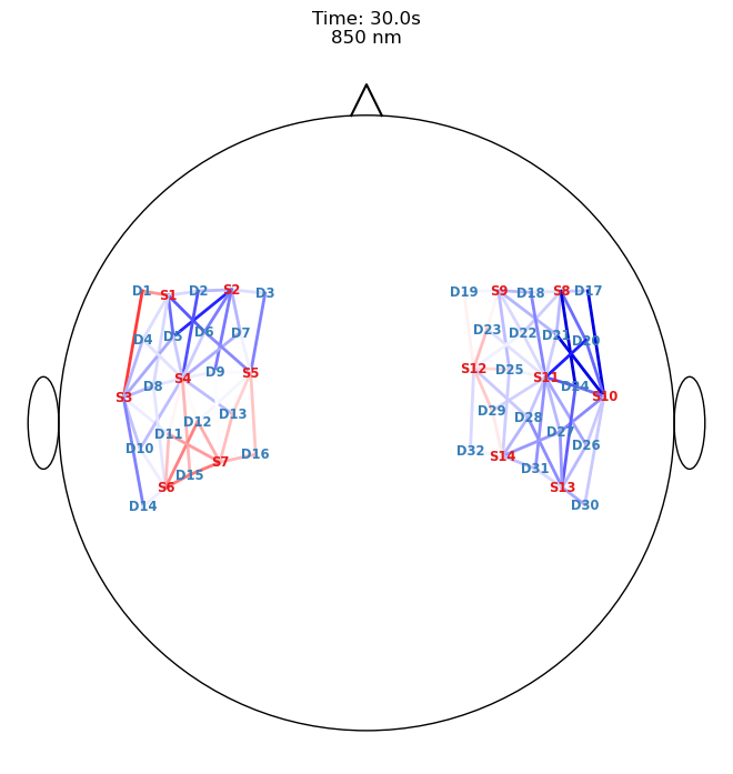
Image Space

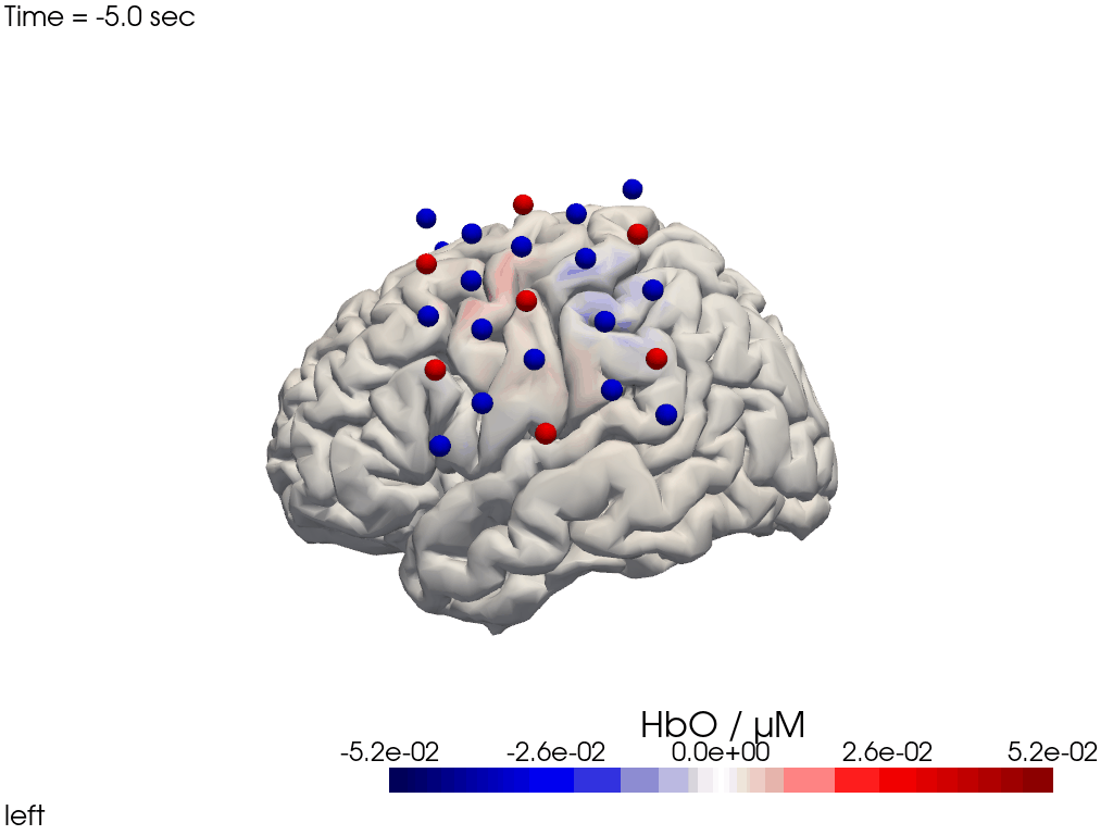
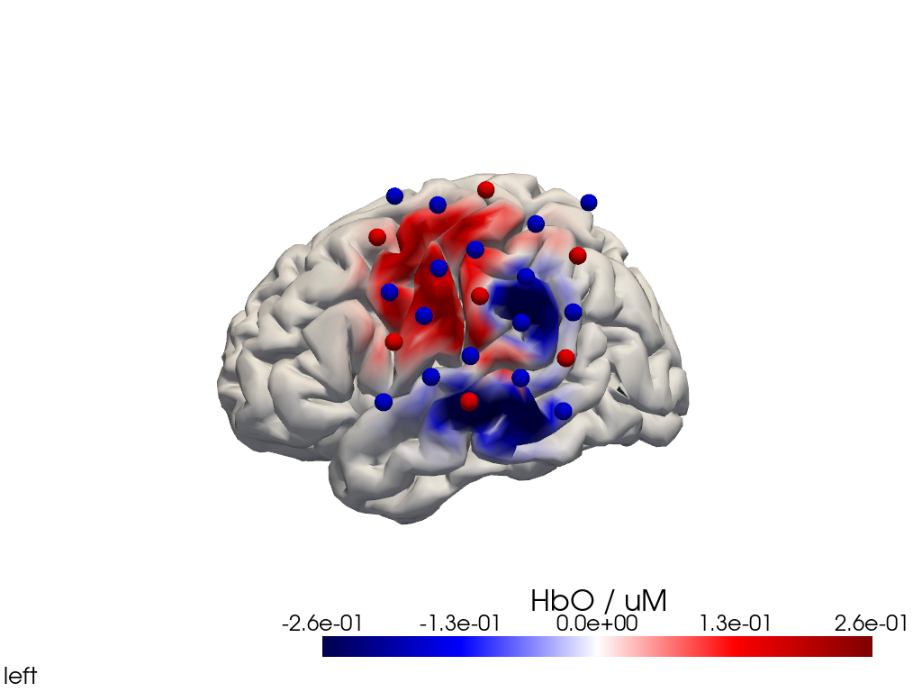
Single-View Animations of Activitations on the Brain

The function cedalion.vis.anatomy.image_recon_view allows to create an animated gif of image-space concentration changes projected on the brain.

filename_view = 'image_recon_view'

# image_recon_view expects input with dimensions
# ("vertex", "chromo", "time") (in that order)
X_ts = img.sel(trial_type="FTapping/Right").rename({"reltime": "time"})
X_ts = X_ts.transpose("vertex", "chromo", "time")

scl = np.percentile(np.abs(X_ts.sel(chromo='HbO')).pint.dequantify(), 99)
clim = (-scl,scl)

cedalion.vis.anatomy.image_recon_view(
    X_ts,  # time series data; can be 2D (static) or 3D (dynamic)
    head_ijk,
    cmap='seismic',
    clim=clim,
    view_type='hbo_brain',
    view_position='left',
    title_str='HbO / µM',
    filename=filename_view,
    SAVE=True,
    time_range=(-5,30,0.5)*units.s,
    fps=6,
    geo3d_plot = geo3d_plot,
    wdw_size = (1024, 768)
)

display_image(f"{filename_view}.gif")

Alternatively, we can just select a single time point and plot activity as a still image at that time. Note the different file suffix (.png).

# selects the nearest time sample at t=4s in X_ts
# note: sel does not accept quantified units
X_ts_plot = X_ts.sel(time=4, method="nearest")

filename_view = 'image_recon_view_still'

cedalion.vis.anatomy.image_recon_view(
    X_ts_plot,  # time series data; can be 2D (static) or 3D (dynamic)
    head_ijk,
    cmap='seismic',
    clim=clim,
    view_type='hbo_brain',
    view_position='left',
    title_str='HbO / µM',
    filename=filename_view,
    SAVE=True,
    time_range=(-5,30,0.5)*units.s,
    fps=6,
    geo3d_plot = geo3d_plot,
    wdw_size = (1024, 768)
)

display_image(f"{filename_view}.png")

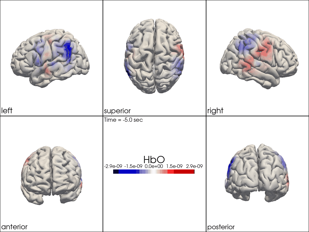
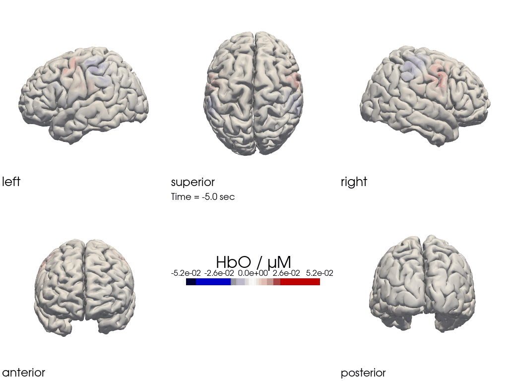
Multi-View Animations of Activitations on the Brain

The function cedalion.vis.anatomy.image_recon_multi_view shows the activity on the brain from all angles as still image or animated across time:

filename_multiview = 'image_recon_multiview'

# prepare data
X_ts = img.sel(trial_type="FTapping/Right").rename({"reltime": "time"})
X_ts = X_ts.transpose("vertex", "chromo", "time")

scl = np.percentile(np.abs(X_ts.sel(chromo='HbO')).pint.dequantify(), 99)
clim = (-scl,scl)

cedalion.vis.anatomy.image_recon_multi_view(
    X_ts,  # time series data; can be 2D (static) or 3D (dynamic)
    head_ijk,
    cmap='seismic',
    clim=clim,
    view_type='hbo_brain',
    title_str='HbO / µM',
    filename=filename_multiview,
    SAVE=True,
    time_range=(-5,30,0.5)*units.s,
    fps=6,
    geo3d_plot = None, #  geo3d_plot
    wdw_size = (1024, 768)
)

display_image(f"{filename_multiview}.gif")

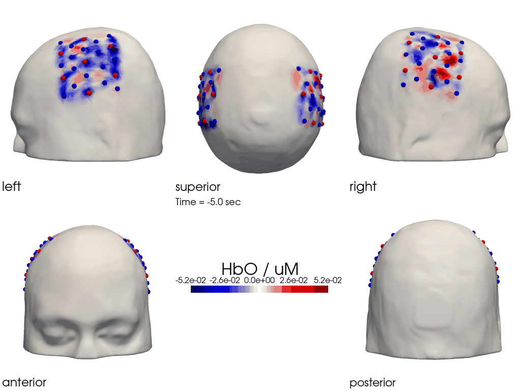
Multi-View Animations of Activitations on the Scalp

This gives us activity on the scalp after recon from all angles as still image or across time

filename_multiview_scalp = 'image_recon_multiview_scalp'

# prepare data
X_ts = img.sel(trial_type="FTapping/Right").rename({"reltime": "time"})
X_ts = X_ts.transpose("vertex", "chromo", "time")

scl = np.percentile(np.abs(X_ts.sel(chromo='HbO')).pint.dequantify(), 99)
clim = (-scl,scl)

cedalion.vis.anatomy.image_recon_multi_view(
    X_ts,  # time series data; can be 2D (static) or 3D (dynamic)
    head_ijk,
    cmap='seismic',
    clim=clim,
    view_type='hbo_scalp',
    title_str='HbO / uM',
    filename=filename_multiview_scalp,
    SAVE=True,
    time_range=(-5,30,0.5)*units.s,
    fps=6,
    geo3d_plot = geo3d_plot,
    wdw_size = (1024, 768)
)

display_image(f"{filename_multiview_scalp}.gif")

Parcel Space

The Schaefer Atlas [SKG+18] as implemented in Cedalion provides nearly 600 labels for different regions of the brain. Each vertex of the brain surface has its correspondng parcel label assigned as a coordinate.

head_ijk.brain.vertices

<xarray.DataArray (label: 15002, ijk: 3)> Size: 360kB
[] 77.71 20.23 74.63 83.52 19.84 69.31 ... 128.0 152.7 100.5 97.28 105.3 87.73
Coordinates:
  * label    (label) int64 120kB 0 1 2 3 4 5 ... 14997 14998 14999 15000 15001
  * parcel   (label) <U44 3MB 'VisCent_ExStr_8_LH' ... 'Background+FreeSurfer...
Dimensions without coordinates: ijk

xarray.DataArray

• label: 15002
• ijk: 3

• [] 77.71 20.23 74.63 83.52 19.84 ... 152.7 100.5 97.28 105.3 87.73

  Magnitude	[[77.714073 20.232582 74.625814] [83.522325 19.841515 69.313221] [84.516588 20.319351 66.886337] ... [98.09373 92.294102 121.835468] [128.025612 152.660339 100.546274] [97.280465 105.252083 87.734898]]
  Units	dimensionless

• Coordinates: (2)
  • label
    (label)
    int64
    0 1 2 3 ... 14998 14999 15000 15001

    array([    0,     1,     2, ..., 14999, 15000, 15001], shape=(15002,))

  • parcel
    (label)
    <U44
    'VisCent_ExStr_8_LH' ... 'Backgr...

    array(['VisCent_ExStr_8_LH', 'VisCent_ExStr_8_LH', 'VisCent_Striate_2_LH', ...,
           'SalVentAttnA_ParMed_6_RH', 'ContA_PFCl_5_RH',
           'Background+FreeSurfer_Defined_Medial_Wall_RH'],
          shape=(15002,), dtype='<U44')

• Indexes: (2)
  • label
    PandasIndex

    PandasIndex(Index([    0,     1,     2,     3,     4,     5,     6,     7,     8,     9,
           ...
           14992, 14993, 14994, 14995, 14996, 14997, 14998, 14999, 15000, 15001],
          dtype='int64', name='label', length=15002))

  • parcel
    PandasIndex

    PandasIndex(Index(['VisCent_ExStr_8_LH', 'VisCent_ExStr_8_LH', 'VisCent_Striate_2_LH',
           'VisCent_Striate_2_LH', 'VisCent_ExStr_8_LH', 'VisCent_Striate_2_LH',
           'VisCent_ExStr_8_LH', 'VisCent_ExStr_8_LH', 'VisCent_Striate_2_LH',
           'VisCent_Striate_2_LH',
           ...
           'SalVentAttnA_ParOper_5_RH', 'DefaultA_PFCm_5_RH',
           'SalVentAttnB_PFCd_2_RH', 'DefaultA_PFCm_4_RH', 'LimbicA_TempPole_8_RH',
           'Background+FreeSurfer_Defined_Medial_Wall_RH', 'ContA_IPS_6_RH',
           'SalVentAttnA_ParMed_6_RH', 'ContA_PFCl_5_RH',
           'Background+FreeSurfer_Defined_Medial_Wall_RH'],
          dtype='object', name='parcel', length=15002))

• Attributes: (0)

To obtain the average hemodynamic response in a parcel, the baseline-subtraced concentration changes of all vertices in a parcel are averaged. As baseline the first sample is used.

# only consider brain vertices in the following.
img_brain = img.sel(vertex=img.is_brain)

# use the first sample along the reltime dimension as baseline
baseline =  img_brain.isel(reltime=0)
img_brain_blsubtracted = img_brain - baseline

display(img_brain_blsubtracted.rename("img_brain_blsubtracted"))

<xarray.DataArray 'img_brain_blsubtracted' (chromo: 2, vertex: 15002,
                                            trial_type: 2, reltime: 154)> Size: 74MB
[µM] 0.0 -1.265e-13 1.859e-12 5.869e-12 ... 2.405e-11 2.357e-11 2.314e-11
Coordinates:
  * chromo      (chromo) <U3 24B 'HbO' 'HbR'
    parcel      (vertex) object 120kB 'VisCent_ExStr_8_LH' ... 'Background+Fr...
    is_brain    (vertex) bool 15kB True True True True ... True True True True
  * reltime     (reltime) float64 1kB -5.038 -4.809 -4.58 ... 29.54 29.77 30.0
  * trial_type  (trial_type) object 16B 'FTapping/Left' 'FTapping/Right'
Dimensions without coordinates: vertex

xarray.DataArray

'img_brain_blsubtracted'

• chromo: 2
• vertex: 15002
• trial_type: 2
• reltime: 154

• [µM] 0.0 -1.265e-13 1.859e-12 ... 2.405e-11 2.357e-11 2.314e-11

  Magnitude

  [[[[0.0 -1.2645415733498582e-13 1.859089573810659e-12 ... 1.0526231078326842e-10 1.0820119726637901e-10 1.1186015255282422e-10] [0.0 -6.395652795432241e-13 5.202912720112764e-14 ... 1.8129263531290172e-11 1.938396968436209e-11 2.0666524413962923e-11]] [[0.0 4.2809417084915885e-14 2.276180598197392e-13 ... 7.740542746897787e-12 7.893067135698053e-12 8.129112197561641e-12] [0.0 -1.3064518330821731e-13 -8.787062039028973e-14 ... -1.6801187606679004e-13 -1.7335857546420076e-13 -1.6595535144485206e-13]] [[0.0 -7.10780927086471e-15 4.158201103252309e-14 ... 3.168835087866459e-12 3.243499399085029e-12 3.3429959415765717e-12] [0.0 -2.940285027306915e-14 -6.5447758698411705e-15 ... 2.402443794703866e-13 2.444239523832545e-13 2.500079613792347e-13]] ... [[0.0 2.0856706539168107e-10 4.5577781417602196e-10 ... 6.524742113573499e-09 6.132424988332867e-09 5.908558471946365e-09] [0.0 -4.008956632944617e-10 -4.690205470234562e-10 ... -7.321359482001068e-09 -7.67920234879585e-09 -7.928290654192526e-09]] [[0.0 -2.0310200703203604e-07 -4.0541876843823946e-07 ... -2.95322139100515e-06 -3.183154965835199e-06 -3.3380170733576178e-06] [0.0 -1.5242777189881065e-07 -3.260295786224903e-07 ... -4.101691857684552e-07 -4.679580523932485e-07 -4.576238380352005e-07]] [[0.0 -4.6204146495168905e-12 -8.016751123732108e-12 ... -1.5608069646015468e-11 -2.3003359423898833e-11 -2.983435398107759e-11] [0.0 -4.184054883865429e-12 -8.083093596940687e-12 ... -2.5894799589759012e-11 -2.8178486635017055e-11 -2.964827279422107e-11]]] [[[0.0 -7.620509000514844e-13 -1.377435895888151e-12 ... 8.93047175490257e-12 9.063331127818334e-12 9.105254151893113e-12] [0.0 -4.069158732197935e-13 -6.847167823096199e-13 ... 5.677527203424127e-12 5.129772997222256e-12 4.859045777799785e-12]] [[0.0 -1.2791200395902616e-13 -2.1537349017799096e-13 ... 3.5322096186229876e-13 3.854926893847004e-13 4.040827516561892e-13] [0.0 -6.073557848536769e-14 -1.264997507090635e-13 ... 6.004796361769511e-13 5.522899421054462e-13 5.159898852955035e-13]] [[0.0 -4.9958644404501077e-14 -9.337988729146856e-14 ... 2.6667955227640233e-13 2.639528555874443e-13 2.6455946575101926e-13] [0.0 -2.4794106458879044e-14 -4.834274720140875e-14 ... 2.4145030779174457e-13 2.2495682876993503e-13 2.1710280337756166e-13]] ... [[0.0 -4.822495414925141e-10 -7.73504643217502e-10 ... -1.5487543186886973e-10 3.845258558690744e-11 1.843078868877718e-10] [0.0 -2.366549884007473e-10 -4.919556541625661e-10 ... 4.87473806760302e-10 4.62968889953598e-10 4.1702603135742164e-10]] [[0.0 1.3540234210631625e-07 2.2943356325902283e-07 ... 6.265042122343218e-07 6.587284328756376e-07 6.436980459157926e-07] [0.0 8.838496448770035e-08 2.2219732902661062e-07 ... -8.27923906871648e-08 -1.264088015689513e-07 -1.698158126494279e-07]] [[0.0 -5.844370583114435e-13 -9.294749870494834e-13 ... 3.538355628078763e-11 3.632708966479805e-11 3.7539301820043935e-11] [0.0 5.706959925803891e-13 2.1806409614417214e-12 ... 2.4053986375358707e-11 2.3574644174255184e-11 2.3144549908927457e-11]]]]

  Units

  micromolar

• Coordinates: (5)
  • chromo
    (chromo)
    <U3
    'HbO' 'HbR'

    array(['HbO', 'HbR'], dtype='<U3')

  • parcel
    (vertex)
    object
    'VisCent_ExStr_8_LH' ... 'Backgr...

    array(['VisCent_ExStr_8_LH', 'VisCent_ExStr_8_LH', 'VisCent_Striate_2_LH',
           ..., 'SalVentAttnA_ParMed_6_RH', 'ContA_PFCl_5_RH',
           'Background+FreeSurfer_Defined_Medial_Wall_RH'],
          shape=(15002,), dtype=object)

  • is_brain
    (vertex)
    bool
    True True True ... True True True

    array([ True,  True,  True, ...,  True,  True,  True], shape=(15002,))

  • reltime
    (reltime)
    float64
    -5.038 -4.809 -4.58 ... 29.77 30.0

    array([-5.038, -4.809, -4.58 , -4.351, -4.122, -3.893, -3.664, -3.435, -3.206,
           -2.977, -2.748, -2.519, -2.29 , -2.061, -1.832, -1.603, -1.374, -1.145,
           -0.916, -0.687, -0.458, -0.229,  0.   ,  0.229,  0.458,  0.687,  0.916,
            1.145,  1.374,  1.603,  1.832,  2.061,  2.29 ,  2.519,  2.748,  2.977,
            3.206,  3.435,  3.664,  3.893,  4.122,  4.351,  4.58 ,  4.809,  5.038,
            5.267,  5.496,  5.725,  5.954,  6.183,  6.412,  6.641,  6.87 ,  7.099,
            7.328,  7.557,  7.786,  8.015,  8.244,  8.473,  8.702,  8.931,  9.16 ,
            9.389,  9.618,  9.847, 10.076, 10.305, 10.534, 10.763, 10.992, 11.221,
           11.45 , 11.679, 11.908, 12.137, 12.366, 12.595, 12.824, 13.053, 13.282,
           13.511, 13.74 , 13.969, 14.198, 14.427, 14.656, 14.885, 15.114, 15.343,
           15.572, 15.801, 16.03 , 16.259, 16.488, 16.717, 16.946, 17.175, 17.404,
           17.633, 17.862, 18.091, 18.32 , 18.549, 18.778, 19.007, 19.236, 19.465,
           19.694, 19.923, 20.152, 20.381, 20.61 , 20.839, 21.068, 21.297, 21.526,
           21.755, 21.984, 22.213, 22.442, 22.671, 22.9  , 23.129, 23.358, 23.587,
           23.816, 24.045, 24.274, 24.503, 24.732, 24.961, 25.19 , 25.419, 25.648,
           25.877, 26.106, 26.335, 26.564, 26.793, 27.022, 27.251, 27.48 , 27.709,
           27.938, 28.167, 28.396, 28.625, 28.854, 29.083, 29.312, 29.541, 29.77 ,
           29.999])

  • trial_type
    (trial_type)
    object
    'FTapping/Left' 'FTapping/Right'

    array(['FTapping/Left', 'FTapping/Right'], dtype=object)

• Indexes: (3)
  • chromo
    PandasIndex

    PandasIndex(Index(['HbO', 'HbR'], dtype='object', name='chromo'))

  • reltime
    PandasIndex

    PandasIndex(Index([             -5.038,              -4.809,               -4.58,
                        -4.351,              -4.122, -3.8930000000000002,
                        -3.664,              -3.435,              -3.206,
           -2.9770000000000003,
           ...
            27.938000000000002,              28.167,              28.396,
                        28.625,  28.854000000000003,  29.083000000000002,
                        29.312,              29.541,               29.77,
            29.999000000000002],
          dtype='float64', name='reltime', length=154))

  • trial_type
    PandasIndex

    PandasIndex(Index(['FTapping/Left', 'FTapping/Right'], dtype='object', name='trial_type'))

• Attributes: (0)

Using parcel labels, vertices belonging to the same brain region can be easily grouped together with the DataArray.groupby function. On these vertex groups many reduction methods can be executed. He we use the function mean() to average over vertices.

Note how the time series dimension changed from vertex to parcel:

# average over parcels
avg_HbO = img_brain_blsubtracted.sel(chromo="HbO").groupby('parcel').mean()
avg_HbR = img_brain_blsubtracted.sel(chromo="HbR").groupby('parcel').mean()

display(avg_HbO.rename("avg_HbO"))

<xarray.DataArray 'avg_HbO' (parcel: 602, trial_type: 2, reltime: 154)> Size: 1MB
[µM] 0.0 4.61e-10 1.547e-09 3.338e-09 ... -6.201e-12 -6.5e-12 -6.656e-12
Coordinates:
    chromo      <U3 12B 'HbO'
  * reltime     (reltime) float64 1kB -5.038 -4.809 -4.58 ... 29.54 29.77 30.0
  * trial_type  (trial_type) object 16B 'FTapping/Left' 'FTapping/Right'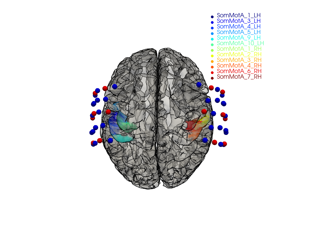
  * parcel      (parcel) object 5kB 'Background+FreeSurfer_Defined_Medial_Wal...

xarray.DataArray

'avg_HbO'

• parcel: 602
• trial_type: 2
• reltime: 154

• [µM] 0.0 4.61e-10 1.547e-09 ... -6.201e-12 -6.5e-12 -6.656e-12

  Magnitude

  [[[0.0 4.610385195608311e-10 1.5469216804720483e-09 ... -1.6766011443287708e-08 -1.5765954838049702e-08 -1.4026350830464665e-08] [0.0 2.725006985906191e-10 6.046528097886086e-10 ... 5.7282212737993365e-09 8.332776723165576e-09 1.2056766855840586e-08]] [[0.0 -1.0361592572316099e-10 -1.252542274193074e-10 ... -2.824960200317262e-09 -3.2662381464783004e-09 -3.790319821945913e-09] [0.0 9.792345163943295e-11 2.460830740234942e-10 ... 2.0676881100889885e-09 1.7441561351480357e-09 1.5386657434587197e-09]] [[0.0 -2.1361601907884144e-10 -3.7619720058316186e-10 ... 3.1294792297069985e-09 3.176960681723657e-09 3.2470853027496228e-09] [0.0 -1.2612733960537852e-10 -2.3511699174247767e-10 ... -1.9463760802903718e-09 -1.7682226211528772e-09 -1.5648804543430967e-09]] ... [[0.0 -4.2716621655353375e-14 9.707504501327666e-14 ... 9.306563952140655e-12 9.52195730767307e-12 9.811263294526792e-12] [0.0 -7.907238558057035e-14 -1.658308945806074e-14 ... 8.544106005788555e-13 8.890192294929402e-13 9.384715232419357e-13]] [[0.0 -4.964974365630908e-13 7.629984346750249e-12 ... -3.0984204082067595e-10 -3.4589344572247674e-10 -3.816681599466045e-10] [0.0 -1.798697716795492e-11 -2.4052209251530153e-11 ... 2.614011841928413e-10 2.313335948103316e-10 2.0544325006973202e-10]] [[0.0 2.97556905909581e-13 7.311436124643988e-13 ... 1.2268814624201478e-11 1.1906874216177196e-11 1.183071495548825e-11] [0.0 -4.568804579321532e-13 -3.7881578355400924e-13 ... -6.2005788157414126e-12 -6.500491148813138e-12 -6.656030975171518e-12]]]

  Units

  micromolar

• Coordinates: (4)
  • chromo
    ()
    <U3
    'HbO'

    array('HbO', dtype='<U3')

  • reltime
    (reltime)
    float64
    -5.038 -4.809 -4.58 ... 29.77 30.0

    array([-5.038, -4.809, -4.58 , -4.351, -4.122, -3.893, -3.664, -3.435, -3.206,
           -2.977, -2.748, -2.519, -2.29 , -2.061, -1.832, -1.603, -1.374, -1.145,
           -0.916, -0.687, -0.458, -0.229,  0.   ,  0.229,  0.458,  0.687,  0.916,
            1.145,  1.374,  1.603,  1.832,  2.061,  2.29 ,  2.519,  2.748,  2.977,
            3.206,  3.435,  3.664,  3.893,  4.122,  4.351,  4.58 ,  4.809,  5.038,
            5.267,  5.496,  5.725,  5.954,  6.183,  6.412,  6.641,  6.87 ,  7.099,
            7.328,  7.557,  7.786,  8.015,  8.244,  8.473,  8.702,  8.931,  9.16 ,
            9.389,  9.618,  9.847, 10.076, 10.305, 10.534, 10.763, 10.992, 11.221,
           11.45 , 11.679, 11.908, 12.137, 12.366, 12.595, 12.824, 13.053, 13.282,
           13.511, 13.74 , 13.969, 14.198, 14.427, 14.656, 14.885, 15.114, 15.343,
           15.572, 15.801, 16.03 , 16.259, 16.488, 16.717, 16.946, 17.175, 17.404,
           17.633, 17.862, 18.091, 18.32 , 18.549, 18.778, 19.007, 19.236, 19.465,
           19.694, 19.923, 20.152, 20.381, 20.61 , 20.839, 21.068, 21.297, 21.526,
           21.755, 21.984, 22.213, 22.442, 22.671, 22.9  , 23.129, 23.358, 23.587,
           23.816, 24.045, 24.274, 24.503, 24.732, 24.961, 25.19 , 25.419, 25.648,
           25.877, 26.106, 26.335, 26.564, 26.793, 27.022, 27.251, 27.48 , 27.709,
           27.938, 28.167, 28.396, 28.625, 28.854, 29.083, 29.312, 29.541, 29.77 ,
           29.999])

  • trial_type
    (trial_type)
    object
    'FTapping/Left' 'FTapping/Right'

    array(['FTapping/Left', 'FTapping/Right'], dtype=object)

  • parcel
    (parcel)
    object
    'Background+FreeSurfer_Defined_M...

    array(['Background+FreeSurfer_Defined_Medial_Wall_LH',
           'Background+FreeSurfer_Defined_Medial_Wall_RH', 'ContA_Cingm_1_LH', ...,
           'VisPeri_StriCal_4_LH', 'VisPeri_StriCal_4_RH', 'VisPeri_StriCal_5_LH'],
          shape=(602,), dtype=object)

• Indexes: (3)
  • reltime
    PandasIndex

    PandasIndex(Index([             -5.038,              -4.809,               -4.58,
                        -4.351,              -4.122, -3.8930000000000002,
                        -3.664,              -3.435,              -3.206,
           -2.9770000000000003,
           ...
            27.938000000000002,              28.167,              28.396,
                        28.625,  28.854000000000003,  29.083000000000002,
                        29.312,              29.541,               29.77,
            29.999000000000002],
          dtype='float64', name='reltime', length=154))

  • trial_type
    PandasIndex

    PandasIndex(Index(['FTapping/Left', 'FTapping/Right'], dtype='object', name='trial_type'))

  • parcel
    PandasIndex

    PandasIndex(Index(['Background+FreeSurfer_Defined_Medial_Wall_LH',
           'Background+FreeSurfer_Defined_Medial_Wall_RH', 'ContA_Cingm_1_LH',
           'ContA_Cingm_1_RH', 'ContA_IPS_1_LH', 'ContA_IPS_1_RH',
           'ContA_IPS_2_LH', 'ContA_IPS_2_RH', 'ContA_IPS_3_LH', 'ContA_IPS_3_RH',
           ...
           'VisPeri_ExStrSup_7_LH', 'VisPeri_StriCal_1_LH', 'VisPeri_StriCal_1_RH',
           'VisPeri_StriCal_2_LH', 'VisPeri_StriCal_2_RH', 'VisPeri_StriCal_3_LH',
           'VisPeri_StriCal_3_RH', 'VisPeri_StriCal_4_LH', 'VisPeri_StriCal_4_RH',
           'VisPeri_StriCal_5_LH'],
          dtype='object', name='parcel', length=602))

• Attributes: (0)

The montage in this dataset covers only parts of the head. Consequently, many brain regions lack significant signal coverage due to the absence of optodes.

To focus on relevant regions, a subset of parcels from the somatosensory and motor regions in both hemispheres is selected.

selected_parcels = [
    "SomMotA_1_LH", "SomMotA_3_LH", "SomMotA_4_LH",
    "SomMotA_5_LH", "SomMotA_9_LH", "SomMotA_10_LH",

    "SomMotA_1_RH", "SomMotA_2_RH", "SomMotA_3_RH",
    "SomMotA_4_RH", "SomMotA_6_RH", "SomMotA_7_RH"
]

The following plot visualizes the montage and the selected parcels:

# map parcel labels to colors
parcel_colors = {
    parcel: p.cm.jet(i / (len(selected_parcels) - 1))
    for i, parcel in enumerate(selected_parcels)
}

plt = pv.Plotter()

vbx.plot_surface(
    plt,
    head_ijk.brain,
    color=np.asarray(
        [
            parcel_colors.get(parcel, (0.8, 0.8, 0.8, 0.3))
            for parcel in head_ijk.brain.vertices.parcel.values
        ]
    ),
    silhouette=True,
)

vbx.plot_labeled_points(plt, geo3d_plot)

plt.add_legend(labels=parcel_colors.items(), face="o", size=(0.3, 0.3))

vbx.camera_at_cog(plt, head_ijk.brain, rpos=(0, 0, 1), up=(0, 1, 0), fit_scene=True)
plt.show()

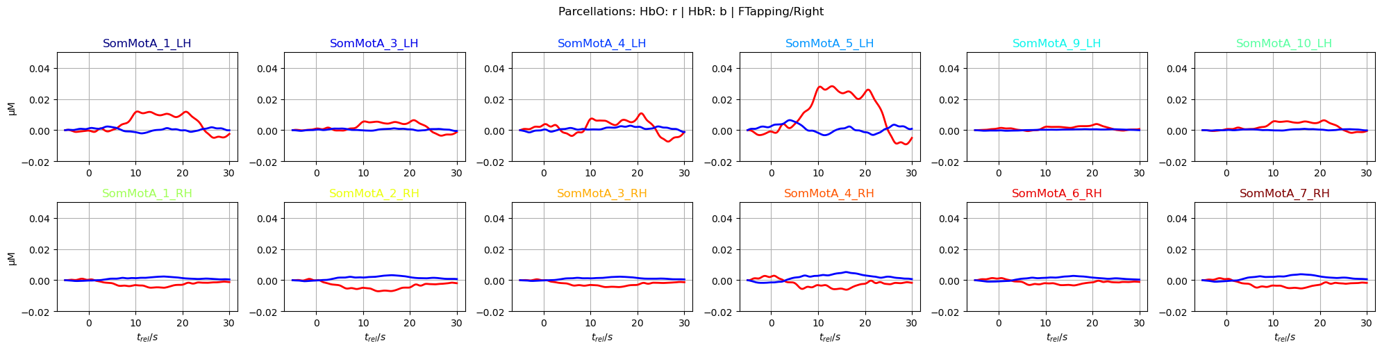
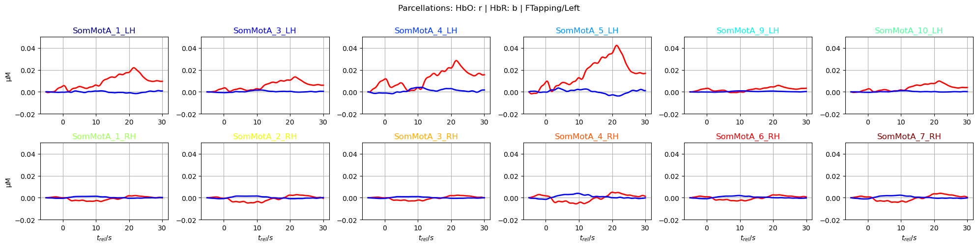
Plot averaged time traces in each parcel for the ‘FTapping/Right’ and ‘FTapping/Left’ conditions:

f,ax = p.subplots(2,6, figsize=(20,5))
ylims = -0.02, 0.05
ax = ax.flatten()
for i_par, par in enumerate(selected_parcels):
    ax[i_par].plot(avg_HbO.sel(parcel = par, trial_type = "FTapping/Right").reltime, avg_HbO.sel(parcel = par, trial_type = "FTapping/Right"), "r", lw=2, ls='-')
    ax[i_par].plot(avg_HbR.sel(parcel = par, trial_type = "FTapping/Right").reltime, avg_HbR.sel(parcel = par, trial_type = "FTapping/Right"), "b", lw=2, ls='-')

    ax[i_par].grid(1)
    ax[i_par].set_title(par, color=parcel_colors[par])
    ax[i_par].set_ylim(*ylims)

    if i_par % 6 == 0:
        ax[i_par].set_ylabel("µM")
    if i_par >=6:
        ax[i_par].set_xlabel("$t_{rel} / s$")

p.suptitle("Parcellations: HbO: r | HbR: b | FTapping/Right", y=1)
p.tight_layout()

f,ax = p.subplots(2,6, figsize=(20,5))
ax = ax.flatten()
for i_par, par in enumerate(selected_parcels):
    ax[i_par].plot(avg_HbO.sel(parcel = par, trial_type = "FTapping/Left").reltime, avg_HbO.sel(parcel = par, trial_type = "FTapping/Left"), "r", lw=2, ls='-')
    ax[i_par].plot(avg_HbR.sel(parcel = par, trial_type = "FTapping/Left").reltime, avg_HbR.sel(parcel = par, trial_type = "FTapping/Left"), "b", lw=2, ls='-')

    ax[i_par].grid(1)
    ax[i_par].set_title(par, color=parcel_colors[par])
    ax[i_par].set_ylim(*ylims)

    if i_par % 6 == 0:
        ax[i_par].set_ylabel("µM")
    if i_par >=6:
        ax[i_par].set_xlabel("$t_{rel} / s$")

p.suptitle("Parcellations: HbO: r | HbR: b | FTapping/Left", y=1)
p.tight_layout()