Fitting a GLM with Gaussian Kernels
Overview
This notebook extends the basic GLM analysis shown in 32_glm_fingertapping_example. It covers:
Advanced design matrices — Gaussian kernel basis functions with cosine drift regressors and average short-channel regressors; long/short channel separation.
Noise model comparison — OLS vs AR-IRLS and their effect on fit quality.
Goodness of fit — median absolute residuals (MAR) and R² scalp maps.
Hypothesis testing — formulating contrasts as linear combinations of Gaussian kernel areas under the curve; t-tests per channel and chromophore.
FDR correction — Benjamini-Hochberg correction of channel-wise p-values.
HRF extraction with uncertainty — predicting per-condition HRF shapes with confidence bands derived from the parameter covariance matrix.
Dataset: cedalion.data.get_fingertappingDOT() — the finger-tapping DOT dataset with a higher-density montage and multiple conditions (finger tapping + ball squeezing).
[1]:
# This cells setups the environment when executed in Google Colab.
try:
    import google.colab
    !curl -s https://raw.githubusercontent.com/ibs-lab/cedalion/dev/scripts/colab_setup.py -o colab_setup.py
    # Select branch with --branch "branch name" (default is "dev")
    %run colab_setup.py
except ImportError:
    pass
[2]:
import cedalion
import cedalion.sigproc.quality as quality
import cedalion.sigproc.motion as motion
import cedalion.sigproc.physio as physio


from cedalion import units
import cedalion.xrutils as xrutils
import cedalion.models.glm as glm
import cedalion.data

import cedalion.vis.blocks as vbx
from cedalion.vis.anatomy import scalp_plot, plot_montage3D
from cedalion.vis.colors import p_values_cmap

import numpy as np
import xarray as xr

import matplotlib.pyplot as p
from statsmodels.stats.multitest import multipletests

xr.set_options(display_expand_data=False)
xrutils.unit_stripping_is_error()
Load Data
[3]:
rec = cedalion.data.get_fingertappingDOT()

# assign better trial_type labels
rec.stim.cd.rename_events(
    {
        "1": "Control",
        "2": "FTapping/Left",
        "3": "FTapping/Right",
        "4": "BallSqueezing/Left",
        "5": "BallSqueezing/Right",
    }
)
[4]:
# count trials
rec.stim.groupby("trial_type")[["trial_type"]].count().rename(
    {"trial_type": "# trials"},
    axis=1,
)
[4]:
| # trials | |
|---|---|
| trial_type | |
| BallSqueezing/Left | 17 |
| BallSqueezing/Right | 16 |
| Control | 65 |
| FTapping/Left | 16 |
| FTapping/Right | 16 |
Trim dataset
Reduce the lenght of the dataset to about 5 minutes. This keeps computing times low for presentation and maintains 3 trials for each condition. Also ignore the BallSqueezing conditions.
[5]:
tmin = 5
tmax = 315

rec.stim = rec.stim[
    (tmin <= rec.stim.onset)
    & (rec.stim.onset <= tmax)
    & (rec.stim.trial_type.isin(["Control", "FTapping/Left", "FTapping/Right"]))
]
rec["amp_cropped"] = rec["amp"].sel(time=slice(tmin,tmax))

# count trials
rec.stim.groupby("trial_type")[["trial_type"]].count().rename(
    {"trial_type": "# trials"},
    axis=1,
)
[5]:
| # trials | |
|---|---|
| trial_type | |
| Control | 10 |
| FTapping/Left | 3 |
| FTapping/Right | 3 |
Preprocessing
apply TDDR and wavelet corrections
remove two known bad channels
transform to concentrations
apply a frequency filter
[6]:
rec["od"] = cedalion.nirs.cw.int2od(rec["amp_cropped"])
rec["od_tddr"] = motion.tddr(rec["od"])
rec["od_wavelet"] = motion.wavelet(rec["od_tddr"])

bad_channels = ['S13D26', 'S14D28']

rec["od_clean"] = rec["od_wavelet"].sel(channel=~rec["od"].channel.isin(bad_channels))

# differential pathlength factors
dpf = xr.DataArray(
    [6, 6],
    dims="wavelength",
    coords={"wavelength": rec["amp"].wavelength},
)

rec["conc"] = cedalion.nirs.cw.od2conc(rec["od_clean"], rec.geo3d, dpf, spectrum="prahl")

# Here we use a lowpass-filter to remove the cardiac component.
# Drift will be modeled in the design matrix.

fmin = 0 * units.Hz
fmax = 0.5 * units.Hz

rec["conc_filtered"] = cedalion.sigproc.frequency.freq_filter(rec["conc"], fmin, fmax)

TS_NAME = "conc_filtered"
[7]:
display(rec[TS_NAME])
<xarray.DataArray 'concentration' (chromo: 2, channel: 98, time: 1352)> Size: 2MB
[µM] 0.8276 0.7548 0.7043 0.6868 0.6978 ... -0.08036 -0.07753 -0.07426 -0.07086
Coordinates:
  * chromo    (chromo) <U3 24B 'HbO' 'HbR'
  * time      (time) float64 11kB 5.046 5.276 5.505 5.734 ... 314.5 314.7 314.9
    samples   (time) int64 11kB 22 23 24 25 26 27 ... 1369 1370 1371 1372 1373
  * channel   (channel) object 784B 'S1D1' 'S1D2' 'S1D4' ... 'S14D31' 'S14D32'
    source    (channel) object 784B 'S1' 'S1' 'S1' 'S1' ... 'S14' 'S14' 'S14'
detector (channel) object 784B 'D1' 'D2' 'D4' 'D5' ... 'D29' 'D31' 'D32'Montage and Channel Distances
[8]:
plot_montage3D(rec["amp"], rec.geo3d)
[9]:
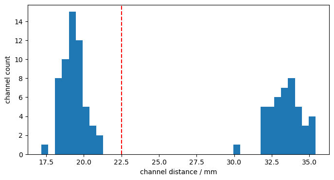
distances = cedalion.nirs.channel_distances(rec["amp"], rec.geo3d)

p.figure(figsize=(8,4))
p.hist(distances, 40)
p.axvline(22.5, c="r", ls="--")
p.xlabel("channel distance / mm")
p.ylabel("channel count");

The montage has longer (3-3.5cm) and shorter (~1.7-2.2cm) distance channels. Define a cut-off at 22.5 mm to define long and short channels.
[10]:
rec["ts_long"], rec["ts_short"] = cedalion.nirs.split_long_short_channels(
    rec[TS_NAME], rec.geo3d, distance_threshold=22.5 * units.mm
)

display(rec["ts_long"])
display(rec["ts_short"])
<xarray.DataArray 'concentration' (chromo: 2, channel: 44, time: 1352)> Size: 952kB
[µM] 0.3715 0.3284 0.2975 0.2849 0.2892 ... 0.006362 0.008495 0.01122 0.01438
Coordinates:
  * chromo    (chromo) <U3 24B 'HbO' 'HbR'
  * time      (time) float64 11kB 5.046 5.276 5.505 5.734 ... 314.5 314.7 314.9
    samples   (time) int64 11kB 22 23 24 25 26 27 ... 1369 1370 1371 1372 1373
  * channel   (channel) object 352B 'S1D6' 'S1D8' 'S2D5' ... 'S14D25' 'S14D27'
    source    (channel) object 352B 'S1' 'S1' 'S2' 'S2' ... 'S13' 'S14' 'S14'
detector (channel) object 352B 'D6' 'D8' 'D5' 'D9' ... 'D28' 'D25' 'D27'<xarray.DataArray 'concentration' (chromo: 2, channel: 54, time: 1352)> Size: 1MB
[µM] 0.8276 0.7548 0.7043 0.6868 0.6978 ... -0.08036 -0.07753 -0.07426 -0.07086
Coordinates:
* chromo (chromo) <U3 24B 'HbO' 'HbR'
* time (time) float64 11kB 5.046 5.276 5.505 5.734 ... 314.5 314.7 314.9
samples (time) int64 11kB 22 23 24 25 26 27 ... 1369 1370 1371 1372 1373
* channel (channel) object 432B 'S1D1' 'S1D2' 'S1D4' ... 'S14D31' 'S14D32'
source (channel) object 432B 'S1' 'S1' 'S1' 'S1' ... 'S14' 'S14' 'S14'
detector (channel) object 432B 'D1' 'D2' 'D4' 'D5' ... 'D29' 'D31' 'D32'Fitting a General Linear Model
Building the Design Matrix
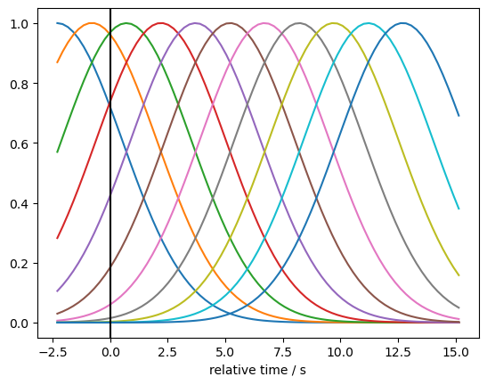
Here we model the HRF with Gaussian kernels. For more modelling choices please refer to the GLM basis functions notebook.
[11]:
gaussian_kernels = glm.basis_functions.GaussianKernels(
    t_pre=2 * units.s,
    t_post=15 * units.s,
    t_delta=1.5 * units.s,
    t_std=2 * units.s,
)

hrf_basis = gaussian_kernels(rec["ts_long"])
for i in range(hrf_basis.sizes["component"]):
    p.plot(hrf_basis.time, hrf_basis[:,i])
    p.xlabel("relative time / s")
p.axvline(0, c="k")
[11]:
<matplotlib.lines.Line2D at 0x7f82e89bd4d0>
Create design matrix from hrf, short channel and drift regressors.
When fitting a GLM to fNIRS data, there are regressors that apply to all channels. Other regressors differ between channel. For example, if one chooses for each channel the closest nearby short-channel to model superficial components, then this regressor differs between channels.
Consequently, the design matrix has two parts: common regressors and channel-wise regressors.
In this example, all short channels are averaged to form a global (mostly) superficial component. The design matrix has only common regressors.
[12]:
dms = (
    glm.design_matrix.hrf_regressors(
        rec["ts_long"],
        rec.stim,
        gaussian_kernels,
    )
    & glm.design_matrix.drift_cosine_regressors(rec[TS_NAME], fmax=0.02 * units.Hz)
    & glm.design_matrix.average_short_channel_regressor(rec["ts_short"])
)
[13]:
display(dms)
display(dms.common)
display(dms.channel_wise)
DesignMatrix(common=['HRF Control 00','HRF Control 01','HRF Control 02','HRF Control 03','HRF Control 04','HRF Control 05','HRF Control 06','HRF Control 07','HRF Control 08','HRF Control 09','HRF Control 10','HRF FTapping/Left 00','HRF FTapping/Left 01','HRF FTapping/Left 02','HRF FTapping/Left 03','HRF FTapping/Left 04','HRF FTapping/Left 05','HRF FTapping/Left 06','HRF FTapping/Left 07','HRF FTapping/Left 08','HRF FTapping/Left 09','HRF FTapping/Left 10','HRF FTapping/Right 00','HRF FTapping/Right 01','HRF FTapping/Right 02','HRF FTapping/Right 03','HRF FTapping/Right 04','HRF FTapping/Right 05','HRF FTapping/Right 06','HRF FTapping/Right 07','HRF FTapping/Right 08','HRF FTapping/Right 09','HRF FTapping/Right 10','Drift Cos 0','Drift Cos 1','Drift Cos 2','Drift Cos 3','Drift Cos 4','Drift Cos 5','Drift Cos 6','Drift Cos 7','Drift Cos 8','Drift Cos 9','Drift Cos 10','Drift Cos 11','short'], channel_wise=[])
<xarray.DataArray (time: 1352, regressor: 46, chromo: 2)> Size: 995kB
0.0 0.0 0.0 0.0 0.0 0.0 0.0 ... 0.9999 0.9999 -0.9999 -0.9999 0.4137 0.03177
Coordinates:
  * time       (time) float64 11kB 5.046 5.276 5.505 5.734 ... 314.5 314.7 314.9
  * regressor  (regressor) <U21 4kB 'HRF Control 00' ... 'short'
  * chromo     (chromo) <U3 24B 'HbO' 'HbR'
    samples    (time) int64 11kB 22 23 24 25 26 27 ... 1369 1370 1371 1372 1373
[]
Visualize the design matrix
[14]:
# select common regressors
dm = dms.common
display(dm)

# using xr.DataArray.plot
f, ax = p.subplots(1,1,figsize=(12,10))
dm.sel(chromo="HbO", time=dm.time < 600).T.plot()
p.title("Shared Regressors")
#p.xticks(rotation=90)
p.show()
<xarray.DataArray (time: 1352, regressor: 46, chromo: 2)> Size: 995kB
0.0 0.0 0.0 0.0 0.0 0.0 0.0 ... 0.9999 0.9999 -0.9999 -0.9999 0.4137 0.03177
Coordinates:
  * time       (time) float64 11kB 5.046 5.276 5.505 5.734 ... 314.5 314.7 314.9
  * regressor  (regressor) <U21 4kB 'HRF Control 00' ... 'short'
  * chromo     (chromo) <U3 24B 'HbO' 'HbR'
    samples    (time) int64 11kB 22 23 24 25 26 27 ... 1369 1370 1371 1372 1373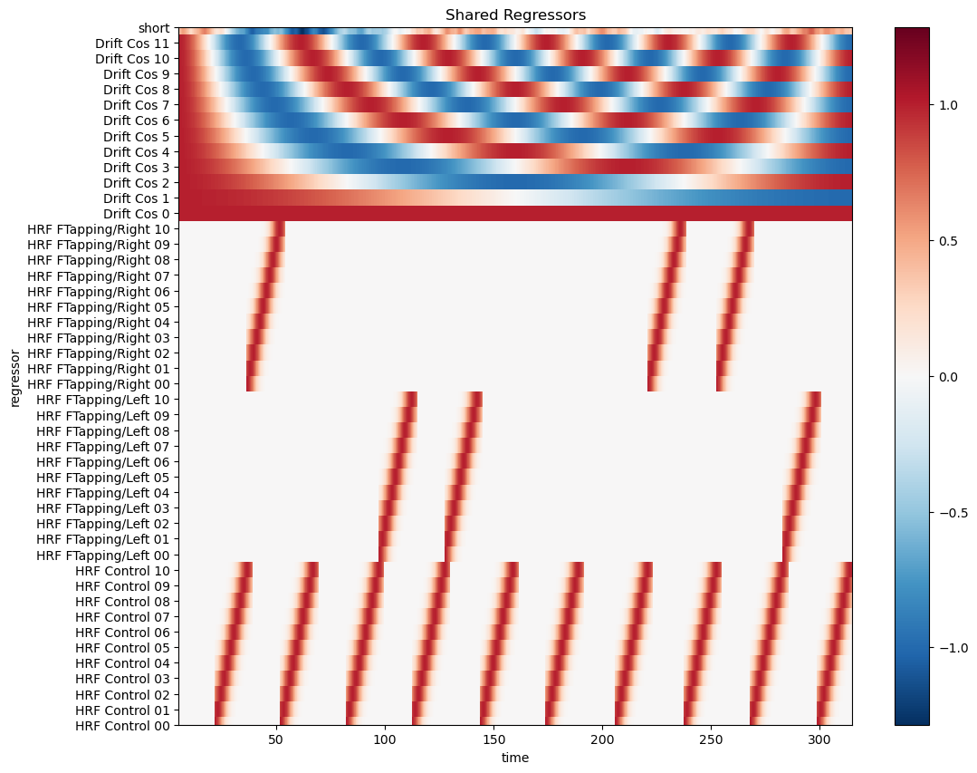
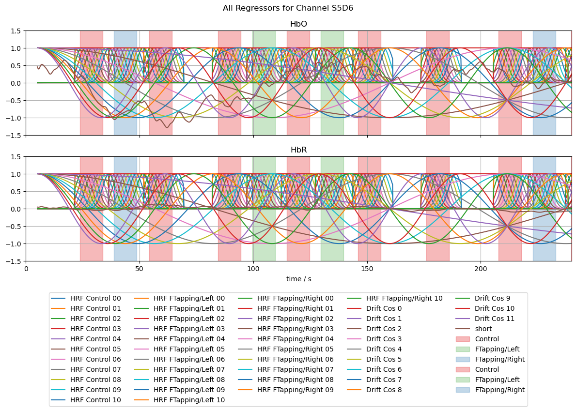
[15]:
# line plots of all regressors
f, ax = p.subplots(2,1,sharex=True, figsize=(12,6))

ch = "S5D6"

for i, chromo in enumerate(["HbO", "HbR"]):
    for reg in dm.regressor.values:
        label = reg if i == 0 else None
        ax[i].plot(dm.time, dm.sel(chromo=chromo, regressor=reg), label=label)

    for cwr in dms.channel_wise:
        for reg in cwr.regressor.values:
            label = reg if i == 0 else None
            ax[i].plot(cwr.time, cwr.sel(chromo=chromo, regressor=reg, channel=ch), label=label)

    vbx.plot_stim_markers(ax[i], rec.stim, y=1)
    ax[i].grid()
    ax[i].set_title(chromo)
    ax[i].set_ylim(-1.5,1.5)
f.suptitle("All Regressors for Channel " + ch)

f.legend(ncol=5, loc="upper center", bbox_to_anchor=(0.5, 0))
ax[0].set_xlim(0,240);
ax[1].set_xlabel("time / s");
f.set_tight_layout(True)
Fitting the Model
Choose between noise_model='ols' and noise_model='ar_irls'.
[16]:
#results = glm.fit(rec["ts_long"], dms, noise_model="ols", max_jobs=-1)
results = glm.fit(rec["ts_long"], dms, noise_model="ar_irls", max_jobs=-1)

display(results)
 98%|█████████▊| 43/44 [02:44<00:03,  3.82s/it]
 98%|█████████▊| 43/44 [01:20<00:01,  1.87s/it]
<xarray.DataArray (channel: 44, chromo: 2)> Size: 704B
<statsmodels.robust.robust_linear_model.RLMResultsWrapper object at 0x7f82e83...
Coordinates:
  * chromo    (chromo) <U3 24B 'HbO' 'HbR'
  * channel   (channel) object 352B 'S1D6' 'S1D8' 'S2D5' ... 'S14D25' 'S14D27'
    source    (channel) object 352B 'S1' 'S1' 'S2' 'S2' ... 'S13' 'S14' 'S14'
    detector  (channel) object 352B 'D6' 'D8' 'D5' 'D9' ... 'D28' 'D25' 'D27'
Attributes:
description: AR_IRLSInspecting Fit Results
The result of the fit is an array of statsmodels result objects. Each contains the fitted parameters and other functionality to inspect fit parameter uncertainty or to perform hypothesis tests.
[17]:
results[0,0].item().params
[17]:
HRF Control 00            0.276679
HRF Control 01           -1.322791
HRF Control 02            3.381821
HRF Control 03           -5.959108
HRF Control 04            7.910174
HRF Control 05           -8.189405
HRF Control 06            6.586288
HRF Control 07           -4.007499
HRF Control 08            1.722847
HRF Control 09           -0.484760
HRF Control 10            0.070155
HRF FTapping/Left 00      0.234327
HRF FTapping/Left 01     -0.918640
HRF FTapping/Left 02      1.663890
HRF FTapping/Left 03     -1.340175
HRF FTapping/Left 04     -0.837867
HRF FTapping/Left 05      3.703104
HRF FTapping/Left 06     -4.886996
HRF FTapping/Left 07      3.755480
HRF FTapping/Left 08     -1.792997
HRF FTapping/Left 09      0.528106
HRF FTapping/Left 10     -0.077728
HRF FTapping/Right 00    -0.858642
HRF FTapping/Right 01     4.243697
HRF FTapping/Right 02   -11.265726
HRF FTapping/Right 03    20.680841
HRF FTapping/Right 04   -28.569771
HRF FTapping/Right 05    30.562608
HRF FTapping/Right 06   -25.349188
HRF FTapping/Right 07    15.793779
HRF FTapping/Right 08    -6.882461
HRF FTapping/Right 09     1.949848
HRF FTapping/Right 10    -0.283047
Drift Cos 0               0.019738
Drift Cos 1              -0.062680
Drift Cos 2              -0.048399
Drift Cos 3              -0.004764
Drift Cos 4               0.098752
Drift Cos 5               0.038450
Drift Cos 6               0.049932
Drift Cos 7               0.015421
Drift Cos 8               0.003108
Drift Cos 9               0.050348
Drift Cos 10              0.032108
Drift Cos 11             -0.038858
short                     0.654660
dtype: float64
separating drift / background regressors and signal
plotting to show model-data fit
Cedalion provides the .sm accessor on arrays of result objects to make accessing the statsmodels functionality easier.
[18]:
display(results.sm.params)
<xarray.DataArray (channel: 44, chromo: 2, regressor: 46)> Size: 32kB
0.2767 -1.323 3.382 -5.959 7.91 ... -0.008269 -0.0007833 0.01253 0.01076 0.2799
Coordinates:
  * regressor  (regressor) object 368B 'HRF Control 00' ... 'short'
  * chromo     (chromo) <U3 24B 'HbO' 'HbR'
  * channel    (channel) object 352B 'S1D6' 'S1D8' 'S2D5' ... 'S14D25' 'S14D27'
    source     (channel) object 352B 'S1' 'S1' 'S2' 'S2' ... 'S13' 'S14' 'S14'
    detector   (channel) object 352B 'D6' 'D8' 'D5' 'D9' ... 'D28' 'D25' 'D27'
Attributes:
description: AR_IRLSThe glm.predict function takes the original time series, the design matrix and the fitted parameters. Using these it predicts the sum of all regressors scaled with the best fitted parameters.
When only a subset of the fitted parameters is provided, only those regressors are considered. This allows to predict the signal or background components separately.
[19]:
predicted = glm.predict(rec["ts_long"], results.sm.params, dms)

predicted_background = glm.predict(
    rec["ts_long"],
    results.sm.params.sel(
        regressor=results.sm.params.regressor.str.startswith("Drift")
        | results.sm.params.regressor.str.startswith("short")
    ),
    dms,
)
predicted_signal = glm.predict(
    rec["ts_long"],
    results.sm.params.sel(regressor=results.sm.params.regressor.str.startswith("HRF")),
    dms,
)

meas_hrf_only = rec["ts_long"].pint.dequantify() - predicted_background
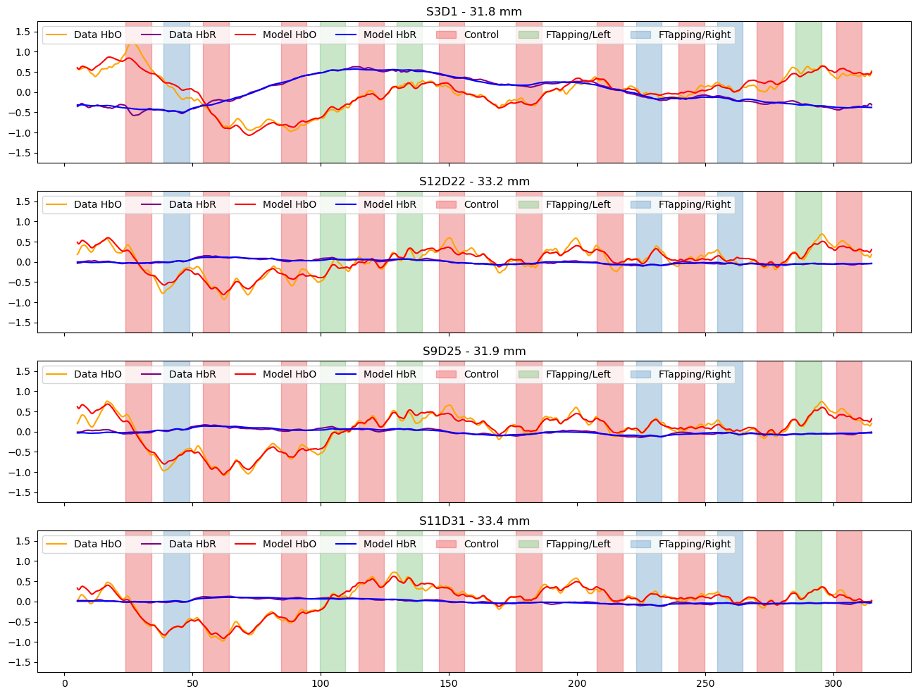
Compare the preprocessed data to the full model
[20]:
channels = ["S3D1", "S12D22", "S9D25", "S11D31"]

f, ax = p.subplots(len(channels),1, figsize=(16, 3*len(channels)), sharex=True)

for i_ch, ch in enumerate(channels):
    ax[i_ch].plot(rec["ts_long"].time, rec["ts_long"].sel(channel=ch, chromo="HbO"), "-", c="orange", label="Data HbO")
    ax[i_ch].plot(rec["ts_long"].time, rec["ts_long"].sel(channel=ch, chromo="HbR"), "-", c="purple", label="Data HbR")
    ax[i_ch].plot(predicted_background.time, predicted.sel(channel=ch, chromo="HbO"), "r-", label="Model HbO")
    ax[i_ch].plot(predicted_background.time, predicted.sel(channel=ch, chromo="HbR"), "b-", label="Model HbR")
    #ax[i_ch].plot(predicted_background.time, predicted_background.sel(channel=ch, chromo="HbO"), "r-", alpha=.5, label="Model Drift HbO")
    #ax[i_ch].plot(predicted_background.time, predicted_background.sel(channel=ch, chromo="HbR"), "b-", alpha=.5, label="Model Drift HbO")
    vbx.plot_stim_markers(ax[i_ch], rec.stim, y=1)
    ax[i_ch].set_title(f"{ch} - {distances.sel(channel=ch).item().magnitude:.1f} mm")
    ax[i_ch].set_ylim(-1.75,1.75)
    ax[i_ch].legend(loc="upper left", ncol=8)
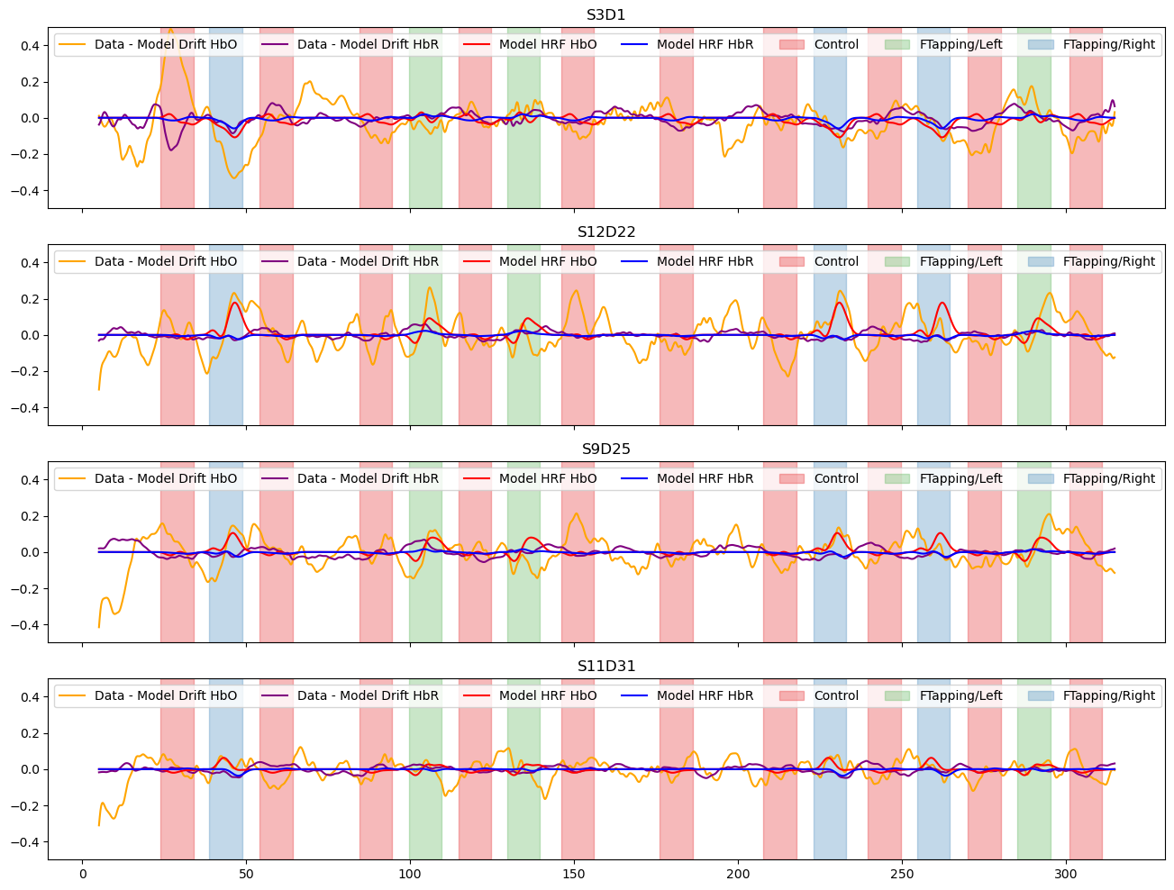
Subtract the components modelled by short and drift regressors and show the fitted activations
[21]:
f, ax = p.subplots(len(channels),1, figsize=(16, 3*len(channels)), sharex=True)

for i_ch, ch in enumerate(channels):
    ax[i_ch].plot(meas_hrf_only.time, meas_hrf_only.sel(channel=ch, chromo="HbO"), "-", c="orange", label="Data - Model Drift HbO" )
    ax[i_ch].plot(meas_hrf_only.time, meas_hrf_only.sel(channel=ch, chromo="HbR"), "-", c="purple", label="Data - Model Drift HbR")
    ax[i_ch].plot(predicted_signal.time, predicted_signal.sel(channel=ch, chromo="HbO"), "r-", label="Model HRF HbO")
    ax[i_ch].plot(predicted_signal.time, predicted_signal.sel(channel=ch, chromo="HbR"), "b-", label="Model HRF HbR")
    vbx.plot_stim_markers(ax[i_ch], rec.stim, y=1)

    ax[i_ch].legend(loc="upper left", ncol=8)
    ax[i_ch].set_title(ch)
    #ax[i_ch].set_ylim(-1.25, 1.25)
    ax[i_ch].set_ylim(-.5, .5)
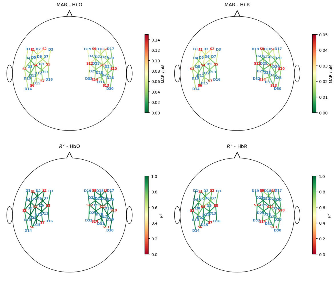
Plot goodness of fit metrics
Here the median absolute residuals (MAR) and \(R^2\) are used.
(Note the scale difference between HbO and HbR for the MAR metric)
[22]:
mar = np.abs(predicted - rec["ts_long"].pint.dequantify()).median("time")

ss_res = ((rec["ts_long"].pint.dequantify() - predicted)**2).sum("time")
ss_tot = ((rec["ts_long"] - rec["ts_long"].mean("time"))**2).pint.dequantify().sum("time")
r2 = (1 - ss_res / ss_tot)

f,ax = p.subplots(2,2, figsize=(12,10))

for i, chromo in enumerate(["HbO", "HbR"]):
    scalp_plot(
        rec["ts_long"],
        rec.geo3d,
        # results.sm.pvalues.sel(regressor=reg, chromo=chromo),
        mar.sel(chromo=chromo),
        ax[0,i],
        cmap="RdYlGn_r",
        vmin=0,
        vmax={"HbO" : 0.15, "HbR" : 0.05}[chromo],
        title=f"MAR - {chromo}",
        cb_label="MAR / µM",
        channel_lw=2,
        optode_labels=True,
        optode_size=24,
    )
    scalp_plot(
        rec["ts_long"],
        rec.geo3d,
        r2.sel(chromo=chromo),
        ax[1,i],
        cmap="RdYlGn",
        vmin=0,
        vmax=1,
        title=f"$R^2$ - {chromo}",
        cb_label="$R^2$",
        channel_lw=2,
        optode_labels=True,
        optode_size=24,
    )

f.set_tight_layout(True)
Hypothesis tests
Performing a hypothesis test requires formulating null hypotheses.
Here H0: the “size of activation” of left or right fingertapping does not differ from the control condition
for simple models with one regressor per condition statsmodels offers and easy interface to formulate H0.
how to express “size of activation” for a model with multiple gaussian kernels?
Formulate H0 as a linear combination of the fitted parameters \(\theta_i\) and a contrast vector \(c_i\) and test if the result deviates from zero:
Here we want to use the area under the HRF as size of the activation
since the model is linear the area under the fitted HRF can be computed by scaling the areas of the gaussian kernels with the fitted parameters
\[\begin{split}A_{HRF} = \begin{pmatrix} \theta_1 \\ \theta_2 \\ \vdots \\ \theta_N \end{pmatrix} \cdot \begin{pmatrix} A_1 \\ A_2 \\ \vdots \\ A_n \end{pmatrix}\end{split}\]Use the area under each regressor as contrast with oppsite signs to formulate which conditions should be compared
restrict area calculation to a time window where the main activation is expected
[23]:
def gaussian_kernel_timewindowed_auc_contrast(
    dms, df_stim, condition1: str, condition2: str, tmin: float, tmax: float
):
    """This function computes contrast vectors based on the time-windowed are of the regressors."""

    time = dms.common.time

    # create two masks, that for each condition contains 1.0 only for
    # time samples between onset+tmin and onset+tmax. All other entries
    # zero
    mask_cond1 = np.zeros(len(time))
    mask_cond2 = np.zeros(len(time))

    for _, row in df_stim.iterrows():
        t1, t2 = row["onset"]+tmin, row["onset"]+tmax
        if row["trial_type"].startswith(condition1):
            mask_cond1[(t1 <= time) & (time <= t2)] = 1.
        if row["trial_type"].startswith(condition2):
            mask_cond2[(t1 <= time) & (time <= t2)] = 1.

    # each gaussian regressor is multiplied with the mask for its condition. This sets
    # all parts of the regressor outside the time window to zero. Through integration the remaining
    # area under the curve is calculated.

    nregressors = dms.common.sizes["regressor"]
    contrast = np.zeros(nregressors)
    for i in range(nregressors):
        if dms.common.regressor.values[i].startswith(f"HRF {condition1}"):
            contrast[i] = np.trapezoid(dms.common[:,i,0]*mask_cond1, dms.common.time)
        if dms.common.regressor.values[i].startswith(f"HRF {condition2}"):
            contrast[i] = - np.trapezoid(dms.common[:,i,0]*mask_cond2, dms.common.time)

    return contrast

hypothesis_labels = [
    "HRF FTapping/Left = HRF Control",
    "HRF FTapping/Right = HRF Control",
]

hypotheses = [
    gaussian_kernel_timewindowed_auc_contrast(dms, rec.stim, "FTapping/Left", "Control", 5, 10),
    gaussian_kernel_timewindowed_auc_contrast(dms, rec.stim, "FTapping/Right", "Control", 5, 10),
]

display(hypotheses)
[array([ -0.38536386,  -1.54846768,  -4.83084777, -11.81761093,
        -22.81664425, -35.12676303, -43.40391258, -43.25178978,
        -34.75902577, -22.41329998, -11.52180284,   0.11269669,
          0.45496975,   1.42568445,   3.50208166,   6.7877193 ,
         10.48759214,  13.0030286 ,  12.99994119,  10.48098719,
          6.78010497,   3.49667564,   0.        ,   0.        ,
          0.        ,   0.        ,   0.        ,   0.        ,
          0.        ,   0.        ,   0.        ,   0.        ,
          0.        ,   0.        ,   0.        ,   0.        ,
          0.        ,   0.        ,   0.        ,   0.        ,
          0.        ,   0.        ,   0.        ,   0.        ,
          0.        ,   0.        ]),
 array([ -0.38536386,  -1.54846768,  -4.83084777, -11.81761093,
        -22.81664425, -35.12676303, -43.40391258, -43.25178978,
        -34.75902577, -22.41329998, -11.52180284,   0.        ,
          0.        ,   0.        ,   0.        ,   0.        ,
          0.        ,   0.        ,   0.        ,   0.        ,
          0.        ,   0.        ,   0.12240493,   0.48687159,
          1.50425073,   3.64608706,   6.97863256,  10.65571472,
         13.06351251,  12.91859368,  10.303389  ,   6.59305506,
          3.36289301,   0.        ,   0.        ,   0.        ,
          0.        ,   0.        ,   0.        ,   0.        ,
          0.        ,   0.        ,   0.        ,   0.        ,
          0.        ,   0.        ])]
Using the calculated contrasts (i.e. hypotheses) perform a t-test in each channel and chromophore using .sm
[24]:
contrast_results = results.sm.t_test(hypotheses)

display(contrast_results)
display(contrast_results[0,0].item())
<xarray.DataArray (channel: 44, chromo: 2)> Size: 704B
                             Test for Constraints                            ...
Coordinates:
  * chromo    (chromo) <U3 24B 'HbO' 'HbR'
  * channel   (channel) object 352B 'S1D6' 'S1D8' 'S2D5' ... 'S14D25' 'S14D27'
    source    (channel) object 352B 'S1' 'S1' 'S2' 'S2' ... 'S13' 'S14' 'S14'
    detector  (channel) object 352B 'D6' 'D8' 'D5' 'D9' ... 'D28' 'D25' 'D27'
Attributes:
    description:  AR_IRLS
<class 'statsmodels.stats.contrast.ContrastResults'>
                             Test for Constraints
==============================================================================
                 coef    std err          z      P>|z|      [0.025      0.975]
------------------------------------------------------------------------------
c0             1.0722      0.886      1.211      0.226      -0.664       2.808
c1             1.4259      0.885      1.611      0.107      -0.309       3.161
==============================================================================
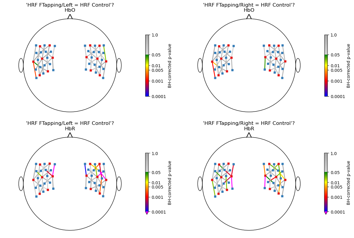
Apply FDR-control and visualize corrected p-values for all channels
[25]:
# create a colormap for p-values
norm, cmap = p_values_cmap()

nhypo = len(hypotheses)
f, ax = p.subplots(2,len(hypotheses),figsize=(6 * nhypo,8))

for i_row, chromo in enumerate(["HbO", "HbR"]):
    for i_hypo, hypo in enumerate(hypotheses):

        # get p_values for all channels and apply fdr correction
        # use Benjamini-Hochberg here
        p_values = contrast_results.sm.p_values().sel(chromo=chromo, hypothesis=i_hypo)
        _, q_values, _, _ = multipletests(p_values, alpha=0.05, method="fdr_bh")

        scalp_plot(
            rec["ts_long"],
            rec.geo3d,
            np.log10(q_values),
            ax[i_row][i_hypo],
            cmap=cmap,
            norm=norm,
            title=f"'{hypothesis_labels[i_hypo]}'?\n{chromo}",
            cb_label="BH-corrected p-value",
            channel_lw=2,
            optode_labels=False,
            cb_ticks_labels=[(np.log10(i), str(i)) for i in [0.0001, 0.001, 0.005, 0.01, 0.05, 1.]],
            optode_size=24,
        )


f.tight_layout()
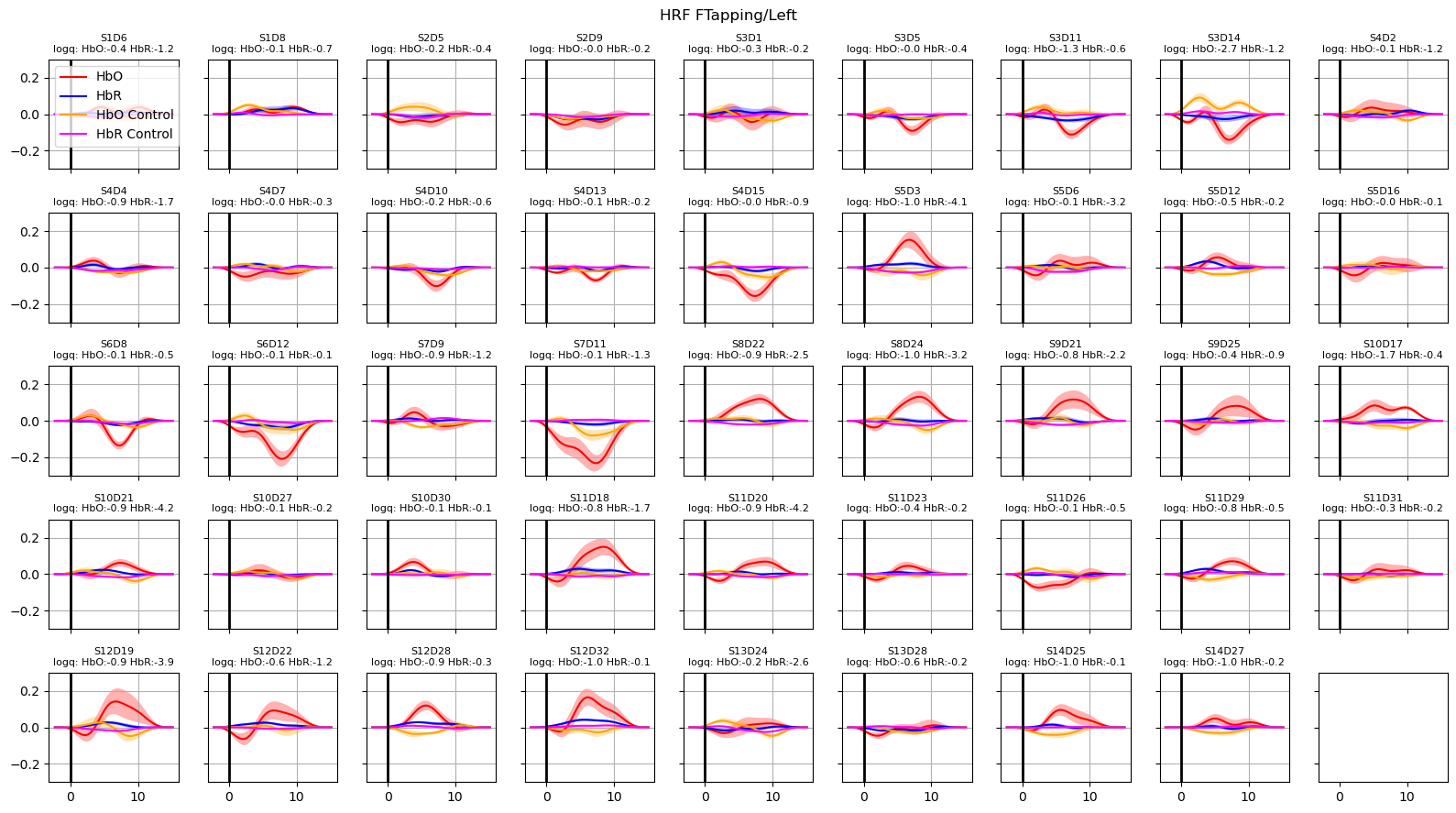
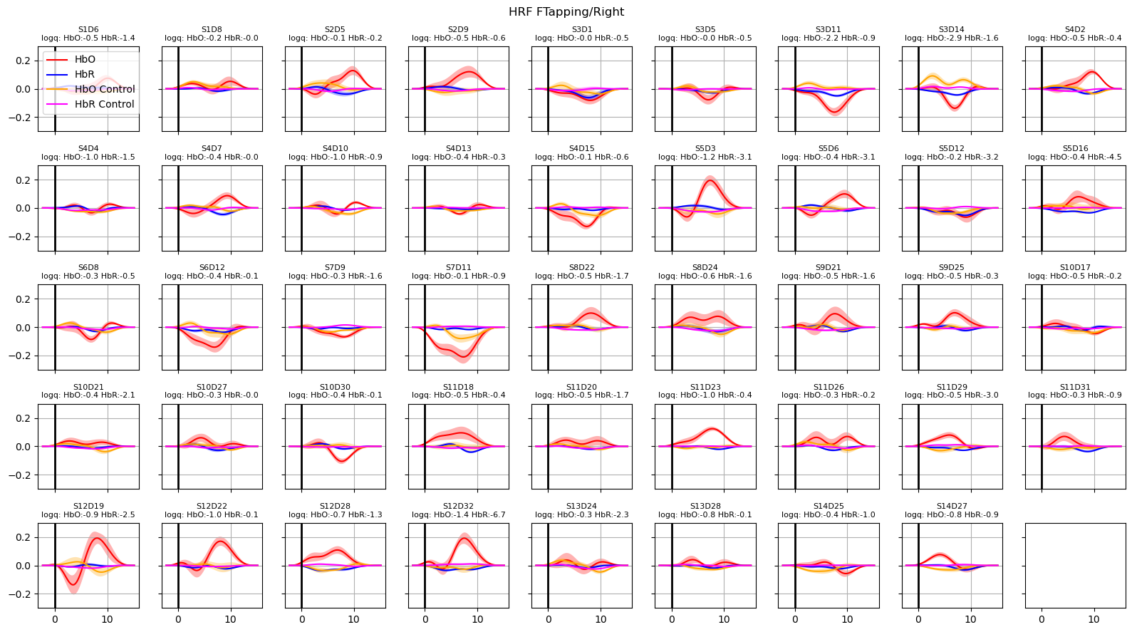
Extract and plot HRFs with uncertainties
for extracting the HRF build a special design matrix
spans only the time of one trial
is not covolved over the stimulus duration (does not apply for gaussian kernels)
[26]:
dms_extract = glm.design_matrix.hrf_extract_regressors(rec["ts_long"], rec.stim, gaussian_kernels)
display(dms_extract.common)
<xarray.DataArray (time: 77, regressor: 33, chromo: 2)> Size: 41kB
1.0 1.0 0.8694 0.8694 0.5698 0.5698 ... 0.1581 0.3804 0.3804 0.6912 0.6912
Coordinates:
  * time       (time) float64 616B -2.294 -2.064 -1.835 ... 14.68 14.91 15.14
  * regressor  (regressor) <U21 3kB 'HRF Control 00' ... 'HRF FTapping/Right 10'
  * chromo     (chromo) <U3 24B 'HbO' 'HbR'
Now predict time series with dms_extract. Additionally account for the uncertainties of the fitted parameters.
Using the covariance matrix of the fitted parameters and a multivariate normal distribution, 10 sets of parameters are sampled around the best fit value. From this ensemble of predictions the mean and std are returned.
[27]:
hrfs_control_mean, hrfs_control_std = glm.predict_with_uncertainty(
    rec["ts_long"],
    results,
    dms_extract,
    results.sm.params.regressor.str.startswith("HRF Control"),
)

for i_hypo, trial_type in enumerate(["HRF FTapping/Left", "HRF FTapping/Right"]):
    hrfs_mean, hrfs_std = glm.predict_with_uncertainty(
        rec["ts_long"],
        results,
        dms_extract,
        results.sm.params.regressor.str.startswith(trial_type),
    )

    p_values_hbo = contrast_results.sm.p_values().sel(chromo="HbO", hypothesis=i_hypo)
    p_values_hbr = contrast_results.sm.p_values().sel(chromo="HbR", hypothesis=i_hypo)

    # apply fdr correction (q-values are shown in captions)
    _, q_values_hbo, _, _ = multipletests(p_values_hbo, alpha=0.05, method="fdr_bh")
    _, q_values_hbr, _, _ = multipletests(p_values_hbr, alpha=0.05, method="fdr_bh")

    channels = hrfs_mean.channel.values

    f, ax = p.subplots(5, 9, figsize=(16, 9), sharex=True, sharey=True)
    ax = ax.flatten()

    for i_ch, ch in enumerate(channels[: len(ax)]):
        q_hbo = np.log10(q_values_hbo[i_ch])
        q_hbr = np.log10(q_values_hbr[i_ch])

        mm_hbo = hrfs_mean.sel(channel=ch, chromo="HbO")
        mm_hbr = hrfs_mean.sel(channel=ch, chromo="HbR")
        ss_hbo = hrfs_std.sel(channel=ch, chromo="HbO")
        ss_hbr = hrfs_std.sel(channel=ch, chromo="HbR")

        ax[i_ch].plot(mm_hbo.time, mm_hbo, "r-", label="HbO")
        ax[i_ch].fill_between(
            mm_hbo.time, mm_hbo - ss_hbo, mm_hbo + ss_hbo, fc="r", alpha=0.3
        )
        ax[i_ch].plot(mm_hbr.time, mm_hbr, "b-", label="HbR")
        ax[i_ch].fill_between(
            mm_hbr.time, mm_hbr - ss_hbr, mm_hbr + ss_hbr, fc="b", alpha=0.3
        )

        mm_hbo = hrfs_control_mean.sel(channel=ch, chromo="HbO")
        mm_hbr = hrfs_control_mean.sel(channel=ch, chromo="HbR")
        ss_hbo = hrfs_control_std.sel(channel=ch, chromo="HbO")
        ss_hbr = hrfs_control_std.sel(channel=ch, chromo="HbR")

        ax[i_ch].plot(mm_hbo.time, mm_hbo, "orange", label="HbO Control")
        ax[i_ch].fill_between(
            mm_hbo.time, mm_hbo - ss_hbo, mm_hbo + ss_hbo, fc="orange", alpha=0.3
        )
        ax[i_ch].plot(mm_hbr.time, mm_hbr, "magenta", label="HbR Control")
        ax[i_ch].fill_between(
            mm_hbr.time, mm_hbr - ss_hbr, mm_hbr + ss_hbr, fc="magenta", alpha=0.3
        )

        ax[i_ch].set_title(
            f"{ch}\nlogq: HbO:{q_hbo:.1f} HbR:{q_hbr:.1f}", fontdict={"fontsize": 8}
        )
        ax[i_ch].set_ylim(-0.3, 0.3)
        ax[i_ch].grid()
        ax[i_ch].axvline(0, c="k", lw=2)
        if i_ch == 0:
            ax[i_ch].legend(loc="upper left")
    f.suptitle(trial_type)
    f.set_tight_layout(True)
References
[28]:
cedalion.bib.dump_to_notebook()
Methods used
| [1] | Tucker2022 | cedalion.io.snirf.read_snirf | Stephen Tucker, Jay Dubb, Sreekanth Kura, Alexander von Lühmann, Robert Franke, Jörn M. Horschig, Samuel Powell, Robert Oostenveld, Michael Lührs, Édouard Delaire, Zahra M. Aghajan, Hanseok Yun, Meryem A. Yücel, Qianqian Fang, Theodore J. Huppert, Blaise deB. Frederick, Luca Pollonini, David A. Boas, and Robert Luke. Introduction to the shared near infrared spectroscopy format. Neurophotonics, 10(1):013507, 2022. doi:10.1117/1.NPh.10.1.013507. |
| [2] | Delpy1988 | cedalion.nirs.cw.int2od, cedalion.nirs.cw.od2conc | D. T. Delpy, M. Cope, P. van der Zee, S. Arridge, S. Wray, and J. Wyatt. Estimation of optical pathlength through tissue from direct time of flight measurement. Physics in Medicine and Biology, 33(12):1433–1442, 1988. doi:10.1088/0031-9155/33/12/008. |
| [3] | Villringer1997 | cedalion.nirs.cw.int2od, cedalion.nirs.cw.od2conc | Arno Villringer and Britton Chance. Non-invasive optical spectroscopy and imaging of human brain function. Trends in Neurosciences, 20(10):435–442, 1997. doi:10.1016/S0166-2236(97)01132-6. |
| [4] | Fishburn2019 | cedalion.sigproc.motion.tddr | Frank A. Fishburn, Ruth S. Ludlum, Chandan J. Vaidya, and Andrei V. Medvedev. Temporal derivative distribution repair (tddr): a motion correction method for fnirs. NeuroImage, 184:171–179, 2019. doi:https://doi.org/10.1016/j.neuroimage.2018.09.025. |
| [5] | Fishburn2018 | cedalion.sigproc.motion.tddr | Frank Fishburn. Tddr. 2018. URL: https://github.com/frankfishburn/TDDR/. |
| [6] | Molavi2012 | cedalion.sigproc.motion.wavelet | Behnam Molavi and Guy A Dumont. Wavelet-based motion artifact removal for functional near-infrared spectroscopy. Physiological Measurement, 33(2):259, 2012. doi:10.1088/0967-3334/33/2/259. |
| [7] | Huppert2009 | cedalion.models.glm.design_matrix.average_short_channel_regressor, cedalion.sigproc.motion.wavelet | Theodore J. Huppert, Solomon G. Diamond, Maria A. Franceschini, and David A. Boas. Homer: a review of time-series analysis methods for near-infrared spectroscopy of the brain. Appl. Opt., 48(10):D280–D298, Apr 2009. doi:https://doi.org/10.1364/AO.48.00D280. |
| [8] | Prahl1998 | cedalion.nirs.common.get_extinction_coefficients | Scott A. Prahl. Optical absorption of hemoglobin. Oregon Medical Laser Center, online resource, 1998. URL: https://omlc.org/spectra/hemoglobin/. |
| [9] | Barker2013 | cedalion.math.ar_irls.ar_irls_GLM, cedalion.models.glm.solve.fit | Jeffrey W. Barker, Ardalan Aarabi, and Theodore J. Huppert. Autoregressive model based algorithm for correcting motion and serially correlated errors in fnirs. Biomed. Opt. Express, 4(8):1366–1379, Aug 2013. doi:10.1364/BOE.4.001366. |