Loading and Inspecting fNIRS Recordings
This notebook shows how to load an fNIRS recording from a SNIRF file and perform a first inspection of the data. Because Cedalion uses the vendor-neutral SNIRF standard, the loading step is identical regardless of which device the data were recorded with — the same two lines of code work for NIRx, Artinis, Gowerlabs, Kernel, and any other SNIRF-compatible system.
After loading, we walk through four inspection steps that are useful for any new dataset:
Channel statistics — distribution of source–detector distances and signal quality (SNR).
Montage — where are the optodes placed on the scalp?
Sensitivity profile — which brain regions are covered by this montage?
Time series — does the raw signal look reasonable?
Prerequisites: familiarity with the Recording container and Cedalion data structures.
Going deeper: links to more detailed notebooks are provided at each step.
[1]:
# This cells setups the environment when executed in Google Colab.
try:
    import google.colab
    !curl -s https://raw.githubusercontent.com/ibs-lab/cedalion/dev/scripts/colab_setup.py -o colab_setup.py
    # Select branch with --branch "branch name" (default is "dev")
    %run colab_setup.py
except ImportError:
    pass
[2]:
# set this flag to True to enable interactive 3D plots
INTERACTIVE_PLOTS = False
[3]:
import cedalion
import cedalion.dot
import cedalion.io
import cedalion.nirs
import cedalion.vis.anatomy
import cedalion.vis.blocks as vbx
import cedalion.sigproc.quality as qlty
import pyvista as pv
import matplotlib.pyplot as plt
from cedalion.geometry.landmarks import normalize_landmarks_labels
import cedalion.data
import numpy as np

if INTERACTIVE_PLOTS:
    pv.set_jupyter_backend("server")
else:
    pv.set_jupyter_backend("static")

# arguments for sensitivity plots:
sensitivity_kwargs = dict(
    cmap="jet",
    scalar_bar_args={
        "title": r"$\log_{10}$ (sensitivity / mm)",
    },
)
Head model
Several of the inspection steps below (montage visualisation, sensitivity profiling) require a head model — a pair of 3-D surface meshes representing the scalp and the cortex together with standard landmark positions. We load it once here and reuse it throughout.
Cedalion ships pre-built head models for the standard atlases Colin27 and ICBM152. For a general introduction into Cedalion headmodels see the Head Models Overview Notebook; for subject-specific analyses you can build a custom head model from an individual MRI - see the Individualized Head Models: MRI Segmentation and TwoSurfaceHeadModel Notebook
[4]:
# Load the Colin27 atlas head model in voxel (ijk) space, then transform it
# into RAS world-space coordinates (mm) for visualisation and geometry operations.
head_ijk = cedalion.dot.get_standard_headmodel("colin27")
head_ras = head_ijk.apply_transform(head_ijk.t_ijk2ras)
Loading and inspecting recordings from different vendors
Any SNIRF file can be loaded with a single function call, regardless of vendor:
rec = cedalion.io.read_snirf("/path/to/your/recording.snirf")
This returns a Recording object that holds the raw amplitude time series, optode geometry, stimulus table, and auxiliary channels. The four inspection steps below — channel statistics, montage, sensitivity profile, and time series — are applied identically to each example dataset.
The following sections walk through example datasets from four different vendors:
NIRx (NIRSport2)
Gowerlabs (LUMO)
Artinis (Octamon)
Kernel (Flow)
NIRx
NIRx provides tabletop and wearable devices with freely configurable otpodes. The example here uses our lab’s own fingertapping example from a HD-Probe that is also shown in other example notebooks.
[5]:
# Load the example NSP2 dataset (downloaded automatically on first use).
# To use your own data, replace this line with:
#   rec = cedalion.io.load_recording("/path/to/your/recording.snirf")
rec = cedalion.data.get_fingertappingDOT()
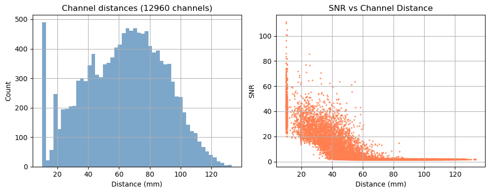
Step 1 — Channel statistics
Before looking at the signal, it is useful to characterise the channel geometry and raw signal quality.
Source–detector distance determines measurement depth: short-separation channels (< 1 cm) primarily sample the scalp; long-separation channels (2.5–4.5 cm) are sensitive to cortical haemodynamics. Above 3.5 cm the sensitivity to cortical haemodynamics improves further, however the amount of received light and thus SNR drastically decreases.
Signal-to-noise ratio (SNR) is a fast first-pass quality check. Channels with very low SNR (typically caused by poor optode contact) should be excluded before further analysis.
For a full quality assessment workflow — including scalp coupling index (SCI), peak-power ratio, and channel pruning — see the signal quality notebook.
[6]:
# calculate the distances for all channels in the recording
distances = cedalion.nirs.channel_distances(rec["amp"], rec.geo3d)
channel_count = len(distances)

# calculate SNR for all channels
snr, _ = qlty.snr(rec["amp"])

# create the plots...
fig, axes = plt.subplots(1, 2, figsize=(10, 4))
# ... a histogram of SNR ...
axes[0].hist(distances, bins=50, alpha=0.7, color="steelblue")
axes[0].set_title(f"Channel distances ({channel_count} channels)")
axes[0].set_xlabel("Distance (mm)")
axes[0].set_ylabel("Count")
axes[0].grid(True)
#... and a scatter plot of SNR vs distance
axes[1].scatter(distances, snr.sel(wavelength=850), alpha=0.7, color="coral", s=2)
axes[1].set_title("SNR vs Channel Distance")
axes[1].set_xlabel("Distance (mm)")
axes[1].set_ylabel("SNR")
axes[1].grid(True)
# show the plots
fig.tight_layout()
plt.show()
/home/runner/miniconda3/envs/cedalion/lib/python3.11/site-packages/xarray/core/variable.py:315: UnitStrippedWarning: The unit of the quantity is stripped when downcasting to ndarray.
  data = np.asarray(data)
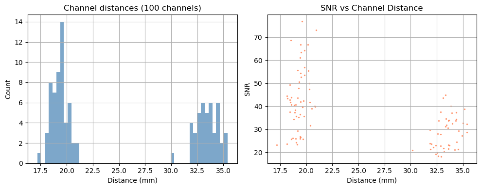
Depending on the measurement setup and vendor all possible source–detector combinations are stored in the SNIRF file, many of which can be too far apart to carry a useful cortical signal. For this example, we retain only channels with a source–detector distance below 3.5 cm.
[7]:
# generate the distance mask
ch_mask = cedalion.nirs.channel_distances(rec["amp"], rec.geo3d) < 3.5 * cedalion.units.cm

# apply the mask to the data
amp = rec["amp"].sel(channel=ch_mask)

# print the number of channels that pass the mask relative to the total number
print(f"Channels passing distance mask: {ch_mask.sum().item()} / {len(ch_mask)}")
Channels passing distance mask: 96 / 100
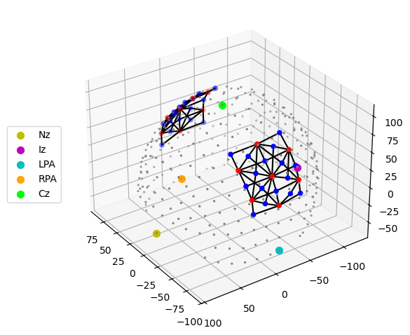
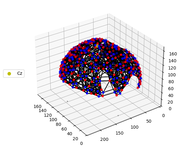
Step 2 — Montage visualisation
Visualising the probe montage on a head surface confirms that the optodes are in anatomically plausible positions and gives an immediate sense of the cortical coverage.
We first plot the raw digitised positions reported in the SNIRF file, then register them to the Colin27 atlas scalp surface. Registration involves two sub-steps:
Landmark normalisation — map vendor-specific landmark labels (e.g.
"Nz","nz","nasion") to a common naming convention so they align with the atlas landmarks.Scalp snapping — rigidly align the digitised positions to the atlas and project each optode onto the nearest point on the scalp mesh.
To learn more about probe registration and co-registration using photogrammetry, see the Photogrammetric Co-Registration Notebook.
[8]:
# Quick 3-D view of the optode positions as stored in the SNIRF file,
# without any registration to a head model.
cedalion.vis.anatomy.plot_montage3D(amp, rec.geo3d)
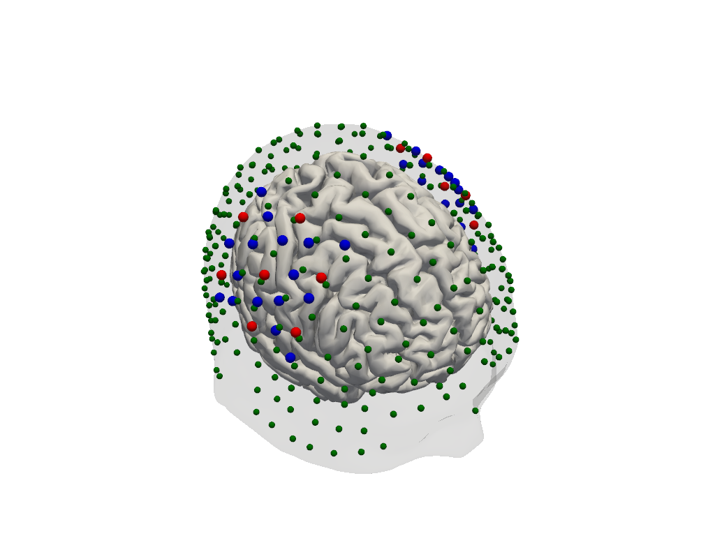
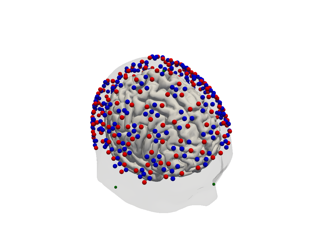
[9]:
# Normalise landmark labels so they match the atlas convention, then
# align and relax the optode positions onto the Colin27 scalp surface.
geo3d = normalize_landmarks_labels(rec.geo3d)
geo3d_snapped, _ = head_ras.align_and_relax_to_scalp(geo3d, rec["amp"])

# Render the scalp (semi-transparent) and cortex together with the registered optodes.
plotter = pv.Plotter()
vbx.plot_surface(plotter, head_ras.scalp, opacity=0.1)
vbx.plot_surface(plotter, head_ras.brain, color="w")
vbx.plot_labeled_points(plotter, geo3d_snapped)
plotter.show()
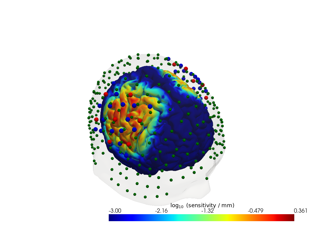
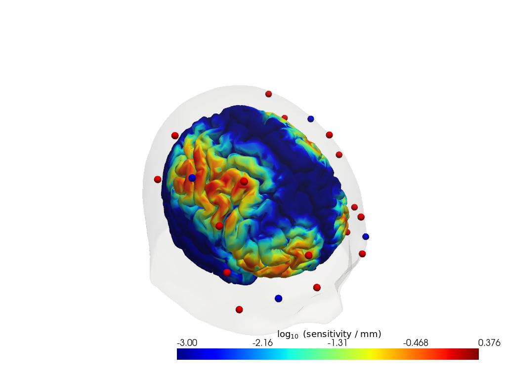
Step 3 — Sensitivity profile
The sensitivity matrix (also called the Jacobian or A matrix) quantifies how much each cortical voxel contributes to each measured channel. Visualising the maximum sensitivity across all channels gives an intuitive map of the cortical area covered by the montage and reveals potential blind spots.
Computing the sensitivity matrix requires running a photon transport simulation (Monte Carlo or FEM), which is computationally expensive. Here we load a pre-computed sensitivity matrix for this dataset. To learn how to compute your own, see the image reconstruction notebook.
[10]:
# Load a pre-computed sensitivity matrix for this dataset at the Colin27 atlas.
Adot = cedalion.data.get_precomputed_sensitivity("fingertappingDOT", "colin27")

# For a spatial overview, take the maximum sensitivity across all channels at 850 nm.
# Restricting to brain vertices avoids scalp contributions dominating the colour scale.
# Log10 is applied because sensitivity varies over several orders of magnitude with depth.
sensitivity = Adot.sel(vertex=Adot.is_brain, wavelength=850).max("channel")

plotter = pv.Plotter()
vbx.plot_surface(plotter, head_ras.scalp, color="w", opacity=0.1)
vbx.plot_surface(plotter, head_ras.brain, color=np.log10(np.clip(sensitivity, 1e-3, 1e1)), **sensitivity_kwargs)
vbx.plot_labeled_points(plotter, geo3d_snapped)
plotter.show()
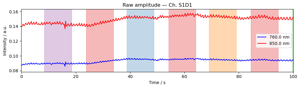
Step 4 — Time series
A quick look at the raw amplitude time series for a single channel confirms that the signal is present and physiologically plausible. Things to look for:
A clear cardiac pulse (~1 Hz oscillation visible in a short window).
No flat sections or sudden jumps that would indicate a saturated or disconnected optode.
Stimulus markers aligned with the expected task timings.
For detailed time series visualisation across many channels — including butterfly plots, quality overlays, and epoch-locked averages — see the Visualization Examples Notebook.
[11]:
ch = amp.channel[0].item()  # pick first channel; replace with a specific channel name if desired

fig, ax = plt.subplots(figsize=(10, 3))
for wl, color in zip(amp.wavelength.values, ["b", "r"]):
    ax.plot(amp.time, amp.sel(channel=ch, wavelength=wl), color=color, label=f"{wl} nm")
ax.set_title(f"Raw amplitude — Ch. {ch}")
ax.set_xlabel("Time / s")
ax.set_ylabel("Intensity / a.u.")
ax.set_xlim(0, 100)
ax.legend()
vbx.plot_stim_markers(ax, rec.stim, y=1)
plt.tight_layout()
plt.show()
Gowerlabs (LUMO)
The Lumo from Gowerlabs is a wearable, modular HD-DOT system. Its tile-based design generates a dense grid of source–detector pairs, including many short-separation channels. Individual optodes cannot be freely configured, but optodes grouped by tiles. Example data here was provided by Gowerlabs.
[12]:
# Load the example LUMO dataset (downloaded automatically on first use).
# To use your own data, replace this line with:
#   rec = cedalion.io.load_recording("/path/to/your/recording.snirf")
rec = cedalion.data.get_lumo_testdataset()
Downloading file 'lumo_testdataset.zip' from 'https://doc.ibs.tu-berlin.de/cedalion/datasets/dev/lumo_testdataset.zip' to '/home/runner/.cache/cedalion/dev'.
Unzipping contents of '/home/runner/.cache/cedalion/dev/lumo_testdataset.zip' to '/home/runner/.cache/cedalion/dev/lumo_testdataset.zip.unzip'
Step 1 — Channel statistics
Before looking at the signal, it is useful to characterise the channel geometry and raw signal quality.
Source–detector distance determines measurement depth: short-separation channels (< 1 cm) primarily sample the scalp; long-separation channels (2.5–4.5 cm) are sensitive to cortical haemodynamics. Above 3.5 cm the sensitivity to cortical haemodynamics improves further, however the amount of received light and thus SNR drastically decreases.
Signal-to-noise ratio (SNR) is a fast first-pass quality check. Channels with very low SNR (typically caused by poor optode contact) should be excluded before further analysis.
For a full quality assessment workflow — including scalp coupling index (SCI), peak-power ratio, and channel pruning — see the signal quality notebook.
[13]:
# calculate the distances for all channels in the recording
distances = cedalion.nirs.channel_distances(rec["amp"], rec.geo3d)
channel_count = len(distances)

# calculate SNR for all channels
snr, _ = qlty.snr(rec["amp"])

# create the plots...
fig, axes = plt.subplots(1, 2, figsize=(10, 4))
# ... a histogram of SNR ...
axes[0].hist(distances, bins=50, alpha=0.7, color="steelblue")
axes[0].set_title(f"Channel distances ({channel_count} channels)")
axes[0].set_xlabel("Distance (mm)")
axes[0].set_ylabel("Count")
axes[0].grid(True)
#... and a scatter plot of SNR vs distance
axes[1].scatter(distances, snr.sel(wavelength=850), alpha=0.7, color="coral", s=2)
axes[1].set_title("SNR vs Channel Distance")
axes[1].set_xlabel("Distance (mm)")
axes[1].set_ylabel("SNR")
axes[1].grid(True)
# show the plots
fig.tight_layout()
plt.show()
/home/runner/miniconda3/envs/cedalion/lib/python3.11/site-packages/xarray/core/variable.py:315: UnitStrippedWarning: The unit of the quantity is stripped when downcasting to ndarray.
  data = np.asarray(data)
Depending on the measurement setup and vendor all possible source–detector combinations are stored in the SNIRF file, many of which can be too far apart to carry a useful cortical signal. For this example, we retain only channels with a source–detector distance below 3.5 cm.
[14]:
# generate the distance mask
ch_mask = cedalion.nirs.channel_distances(rec["amp"], rec.geo3d) < 3.5 * cedalion.units.cm

# apply the mask to the data
amp = rec["amp"].sel(channel=ch_mask)

# print the number of channels that pass the mask relative to the total number
print(f"Channels passing distance mask: {ch_mask.sum().item()} / {len(ch_mask)}")
Channels passing distance mask: 2069 / 12960
Step 2 — Montage visualisation
Visualising the probe montage on a head surface confirms that the optodes are in anatomically plausible positions and gives an immediate sense of the cortical coverage.
We first plot the raw digitised positions reported in the SNIRF file, then register them to the Colin27 atlas scalp surface. Registration involves two sub-steps:
Landmark normalisation — map vendor-specific landmark labels (e.g.
"Nz","nz","nasion") to a common naming convention so they align with the atlas landmarks.Scalp snapping — rigidly align the digitised positions to the atlas and project each optode onto the nearest point on the scalp mesh.
To learn more about probe registration and co-registration using photogrammetry, see the Photogrammetric Co-Registration Notebook.
[15]:
# Quick 3-D view of the optode positions as stored in the SNIRF file,
# without any registration to a head model.
cedalion.vis.anatomy.plot_montage3D(amp, rec.geo3d)
[16]:
# Normalise landmark labels so they match the atlas convention, then
# rigidly align and snap the optode positions onto the Colin27 scalp surface.
geo3d = normalize_landmarks_labels(rec.geo3d)
geo3d_snapped, _ = head_ras.align_and_relax_to_scalp(geo3d, amp)

# Render the scalp (semi-transparent) and cortex together with the registered optodes.
Plotter = pv.Plotter()
vbx.plot_surface(Plotter, head_ras.scalp, opacity=0.1)
vbx.plot_surface(Plotter, head_ras.brain, color="w")
vbx.plot_labeled_points(Plotter, geo3d_snapped)
Plotter.show()
Step 3 — Sensitivity profile
The sensitivity matrix (also called the Jacobian or A matrix) quantifies how much each cortical voxel contributes to each measured channel. Visualising the maximum sensitivity across all channels gives an intuitive map of the cortical area covered by the montage and reveals potential blind spots.
Computing the sensitivity matrix requires running a photon transport simulation (Monte Carlo or FEM), which is computationally expensive. Here we load a pre-computed sensitivity matrix for this dataset. To learn how to compute your own, see the image reconstruction notebook.
[17]:
# Load a pre-computed sensitivity matrix for this dataset at the Colin27 atlas.
Adot = cedalion.data.get_precomputed_sensitivity("lumo_testdataset", "colin27")

# For a spatial overview, take the maximum sensitivity across all channels at 850 nm.
# Restricting to brain vertices avoids scalp contributions dominating the colour scale.
# Log10 is applied because sensitivity varies over several orders of magnitude with depth.
sensitivity = Adot.sel(vertex=Adot.is_brain, wavelength=850).max("channel")

Plotter = pv.Plotter()
vbx.plot_surface(Plotter, head_ras.scalp, color="w", opacity=0.5)
vbx.plot_surface(Plotter, head_ras.brain, color=np.log10(np.clip(sensitivity, 1e-3, 1e1)), **sensitivity_kwargs)
vbx.plot_labeled_points(Plotter, geo3d_snapped)
Plotter.show()
Downloading file 'sensitivity_lumo_testdataset_colin27.nc' from 'https://doc.ibs.tu-berlin.de/cedalion/datasets/dev/sensitivity_lumo_testdataset_colin27.nc' to '/home/runner/.cache/cedalion/dev'.
Step 4 — Time series
A quick look at the raw amplitude time series for a single channel confirms that the signal is present and physiologically plausible. Things to look for:
A clear cardiac pulse (~1 Hz oscillation visible in a short window).
No flat sections or sudden jumps that would indicate a saturated or disconnected optode.
Stimulus markers aligned with the expected task timings.
For detailed time series visualisation across many channels — including butterfly plots, quality overlays, and epoch-locked averages — see the Visualization Examples Notebook.
[18]:
ch = amp.channel[0].item()  # pick first channel; replace with a specific channel name if desired

fig, ax = plt.subplots(figsize=(10, 3))
for wl, color in zip(amp.wavelength.values, ["b", "r"]):
    ax.plot(amp.time, amp.sel(channel=ch, wavelength=wl), color=color, label=f"{wl} nm")
ax.set_title(f"Raw amplitude — Ch. {ch}")
ax.set_xlabel("Time / s")
ax.set_ylabel("Intensity / a.u.")
ax.set_xlim(0, 100)
ax.legend()
vbx.plot_stim_markers(ax, rec.stim, y=1)
plt.tight_layout()
plt.show()
Artinis
Artinis provides wearable devices with freely configurable otpodes. Example data here was taken from: Ajra et al. (2026). Multimodal dataset from the CMx7-MM Experiment. OpenNeuro.
[19]:
# To use your own data, replace this line with:
#   rec = cedalion.io.load_recording("/path/to/your/recording.snirf")
rec = cedalion.data.get_artinis_testdataset()
Downloading file 'artinis_testdataset.zip' from 'https://doc.ibs.tu-berlin.de/cedalion/datasets/dev/artinis_testdataset.zip' to '/home/runner/.cache/cedalion/dev'.
Unzipping contents of '/home/runner/.cache/cedalion/dev/artinis_testdataset.zip' to '/home/runner/.cache/cedalion/dev/artinis_testdataset.zip.unzip'
[20]:
# correct wrong units in SNIRF meta-data
rec.geo3d = rec.geo3d.pint.dequantify().pint.quantify("cm").pint.to("mm")
Step 1 — Channel statistics
Before looking at the signal, it is useful to characterise the channel geometry and raw signal quality.
Source–detector distance determines measurement depth: short-separation channels (< 1 cm) primarily sample the scalp; long-separation channels (2.5–4.5 cm) are sensitive to cortical haemodynamics. Above 3.5 cm the sensitivity to cortical haemodynamics improves further, however the amount of received light and thus SNR drastically decreases.
Signal-to-noise ratio (SNR) is a fast first-pass quality check. Channels with very low SNR (typically caused by poor optode contact) should be excluded before further analysis.
For a full quality assessment workflow — including scalp coupling index (SCI), peak-power ratio, and channel pruning — see the signal quality notebook.
[21]:
# calculate the distances for all channels in the recording
distances = cedalion.nirs.channel_distances(rec["amp"], rec.geo3d)
channel_count = len(distances)

# calculate SNR for all channels
snr, _ = qlty.snr(rec["amp"])

# create the plots...
fig, axes = plt.subplots(1, 2, figsize=(10, 4))
# ... a histogram of SNR ...
axes[0].hist(distances, bins=50, alpha=0.7, color="steelblue")
axes[0].set_title(f"Channel distances ({channel_count} channels)")
axes[0].set_xlabel("Distance (mm)")
axes[0].set_ylabel("Count")
axes[0].grid(True)
#... and a scatter plot of SNR vs distance
axes[1].scatter(distances, snr.sel(wavelength=760), alpha=0.7, color="coral", s=2)
axes[1].set_title("SNR vs Channel Distance")
axes[1].set_xlabel("Distance (mm)")
axes[1].set_ylabel("SNR")
axes[1].grid(True)
# show the plots
fig.tight_layout()
plt.show()
/home/runner/miniconda3/envs/cedalion/lib/python3.11/site-packages/xarray/core/variable.py:315: UnitStrippedWarning: The unit of the quantity is stripped when downcasting to ndarray.
  data = np.asarray(data)
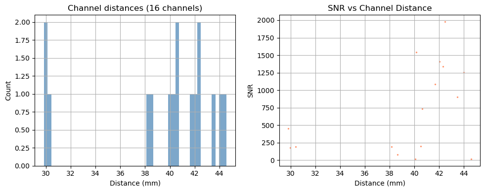
Depending on the measurement setup and vendor all possible source–detector combinations are stored in the SNIRF file, many of which can be too far apart to carry a useful cortical signal. For this example, we retain only channels with a source–detector distance below 3.5 cm.
[22]:
# generate the distance mask
ch_mask = cedalion.nirs.channel_distances(rec["amp"], rec.geo3d) < 3.5 * cedalion.units.cm

# apply the mask to the data
amp = rec["amp"].sel(channel=ch_mask)

# print the number of channels that pass the mask relative to the total number
print(f"Channels passing distance mask: {ch_mask.sum().item()} / {len(ch_mask)}")
Channels passing distance mask: 3 / 16
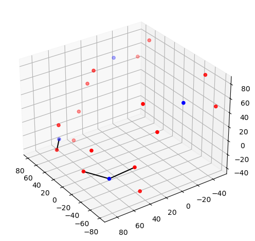
Step 2 — Montage visualisation
Visualising the probe montage on a head surface confirms that the optodes are in anatomically plausible positions and gives an immediate sense of the cortical coverage.
We first plot the raw digitised positions reported in the SNIRF file, then register them to the Colin27 atlas scalp surface. Registration involves two sub-steps:
Landmark normalisation — map vendor-specific landmark labels (e.g.
"Nz","nz","nasion") to a common naming convention so they align with the atlas landmarks.Scalp snapping — rigidly align the digitised positions to the atlas and project each optode onto the nearest point on the scalp mesh.
To learn more about probe registration and co-registration using photogrammetry, see the Photogrammetric Co-Registration Notebook.
[23]:
# Quick 3-D view of the optode positions as stored in the SNIRF file,
# without any registration to a head model.
cedalion.vis.anatomy.plot_montage3D(amp, rec.geo3d)
[24]:
# The dataset does not contain landmark positions. Optode positions appear to be
# registered to the Colin27 atlas.
#geo3d = normalize_landmarks_labels(rec.geo3d)

# rename coordinate reference system
geo3d = rec.geo3d.points.set_crs("mni")
# snap the optode positions onto the Colin27 scalp surface.
geo3d_snapped = head_ras.scalp.snap(geo3d)

# Render the scalp (semi-transparent) and cortex together with the registered optodes.
plotter = pv.Plotter()
vbx.plot_surface(plotter, head_ras.scalp, opacity=0.1)
vbx.plot_surface(plotter, head_ras.brain, color="w")
vbx.plot_labeled_points(plotter, geo3d_snapped)
plotter.show()

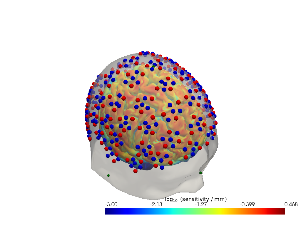
Step 3 — Sensitivity profile
The sensitivity matrix (also called the Jacobian or A matrix) quantifies how much each cortical voxel contributes to each measured channel. Visualising the maximum sensitivity across all channels gives an intuitive map of the cortical area covered by the montage and reveals potential blind spots.
Computing the sensitivity matrix requires running a photon transport simulation (Monte Carlo or FEM), which is computationally expensive. Here we load a pre-computed sensitivity matrix for this dataset. To learn how to compute your own, see the image reconstruction notebook.
[25]:
# Load a pre-computed sensitivity matrix for this dataset at the Colin27 atlas.
Adot = cedalion.data.get_precomputed_sensitivity("artinis_testdataset", "colin27")

# For a spatial overview, take the maximum sensitivity across all channels at 850 nm.
# Restricting to brain vertices avoids scalp contributions dominating the colour scale.
# Log10 is applied because sensitivity varies over several orders of magnitude with depth.
sensitivity = Adot.sel(vertex=Adot.is_brain, wavelength=850).max("channel")

plotter = pv.Plotter()
vbx.plot_surface(plotter, head_ras.scalp, color="w", opacity=0.1)
vbx.plot_surface(plotter, head_ras.brain, color=np.log10(np.clip(sensitivity, 1e-3, 1e1)), **sensitivity_kwargs)
vbx.plot_labeled_points(plotter, geo3d_snapped)
plotter.show()
Downloading file 'sensitivity_artinis_testdataset_colin27.nc' from 'https://doc.ibs.tu-berlin.de/cedalion/datasets/dev/sensitivity_artinis_testdataset_colin27.nc' to '/home/runner/.cache/cedalion/dev'.
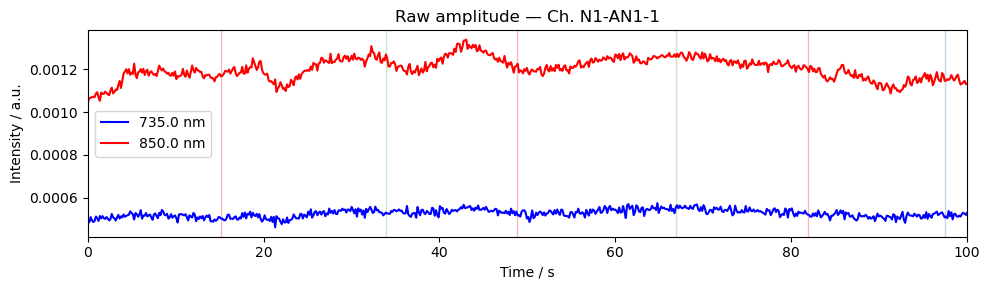
Step 4 — Time series
A quick look at the raw amplitude time series for a single channel confirms that the signal is present and physiologically plausible. Things to look for:
A clear cardiac pulse (~1 Hz oscillation visible in a short window).
No flat sections or sudden jumps that would indicate a saturated or disconnected optode.
Stimulus markers aligned with the expected task timings.
For detailed time series visualisation across many channels — including butterfly plots, quality overlays, and epoch-locked averages — see the Visualization Examples Notebook.
[26]:
ch = amp.channel[0].item()  # pick first channel; replace with a specific channel name if desired

fig, ax = plt.subplots(figsize=(10, 3))
for wl, color in zip(amp.wavelength.values, ["b", "r", "c"]):
    ax.plot(amp.time, amp.sel(channel=ch, wavelength=wl), color=color, label=f"{wl} nm")
ax.set_title(f"Raw amplitude — Ch. {ch}")
ax.set_xlabel("Time / s")
ax.set_ylabel("Intensity / a.u.")
ax.set_xlim(0, 100)
ax.legend()
vbx.plot_stim_markers(ax, rec.stim, y=1)
plt.tight_layout()
plt.show()
Kernel
Kernel provides a wearable modular helmet, the “Flow”, which is a high-density TD-fNIRS system designed for wearable, everyday use. Example data here is taken from the dataset published by Dubois et al. on OpenNeuro.
[27]:
# Load the example NSP2 dataset (downloaded automatically on first use).
# To use your own data, replace this line with:
#   rec = cedalion.io.load_recording("/path/to/your/recording.snirf")
rec = cedalion.data.get_kernel_testdataset()
Downloading file 'kernel_testdataset.zip' from 'https://doc.ibs.tu-berlin.de/cedalion/datasets/dev/kernel_testdataset.zip' to '/home/runner/.cache/cedalion/dev'.
Unzipping contents of '/home/runner/.cache/cedalion/dev/kernel_testdataset.zip' to '/home/runner/.cache/cedalion/dev/kernel_testdataset.zip.unzip'
Step 1 — Channel statistics
Before looking at the signal, it is useful to characterise the channel geometry and raw signal quality. Note, that this time we are looking at data from a time domain (TD) fNIRS device.
Source–detector distance determines measurement depth: short-separation channels (< 1 cm) primarily sample the scalp; longer-separation channels are increasingly sensitive to cortical haemodynamics. Above 3.5 cm, cortical sensitivity improves further, but the amount of received light — and thus SNR — decreases sharply. In TD-fNIRS, depth sensitivity can be enhanced by various strategies, including gating to late-arriving photons that have traveled longer paths through deeper tissue. In this example we do not exploit this capability; instead, we use the 0th moment (total detected intensity), treating the TD-SNIRF data equivalently to continuous-wave measurements
Signal-to-noise ratio (SNR) is a fast first-pass quality check. Channels with very low SNR (typically caused by poor optode contact) should be excluded before further analysis.
For a full quality assessment workflow — including scalp coupling index (SCI), peak-power ratio, and channel pruning — see the signal quality notebook.
[28]:
# calculate the distances for all channels in the recording
distances = cedalion.nirs.channel_distances(rec["amp"], rec.geo3d)
channel_count = len(distances)

# calculate SNR for all channels
snr, _ = qlty.snr(rec["amp"])

# create the plots...
fig, axes = plt.subplots(1, 2, figsize=(10, 4))
# ... a histogram of SNR ...
axes[0].hist(distances, bins=50, alpha=0.7, color="steelblue")
axes[0].set_title(f"Channel distances ({channel_count} channels)")
axes[0].set_xlabel("Distance (mm)")
axes[0].set_ylabel("Count")
axes[0].grid(True)
#... and a scatter plot of SNR vs distance
axes[1].scatter(distances, snr.sel(wavelength=905), alpha=0.7, color="coral", s=2)
axes[1].set_title("SNR vs Channel Distance")
axes[1].set_xlabel("Distance (mm)")
axes[1].set_ylabel("SNR")
axes[1].grid(True)
# show the plots
fig.tight_layout()
plt.show()
/home/runner/miniconda3/envs/cedalion/lib/python3.11/site-packages/xarray/core/variable.py:315: UnitStrippedWarning: The unit of the quantity is stripped when downcasting to ndarray.
  data = np.asarray(data)
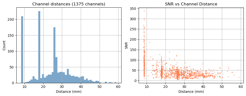
Depending on the measurement setup and vendor all possible source–detector combinations are stored in the SNIRF file, many of which can be too far apart to carry a useful cortical signal. For this example, we retain only channels with a source–detector distance below 3.5 cm.
[29]:
# generate the distance mask
ch_mask = cedalion.nirs.channel_distances(rec["amp"], rec.geo3d) < 3.5 * cedalion.units.cm

# apply the mask to the data
amp = rec["amp"].sel(channel=ch_mask)

# print the number of channels that pass the mask relative to the total number
print(f"Channels passing distance mask: {ch_mask.sum().item()} / {len(ch_mask)}")
Channels passing distance mask: 1164 / 1375
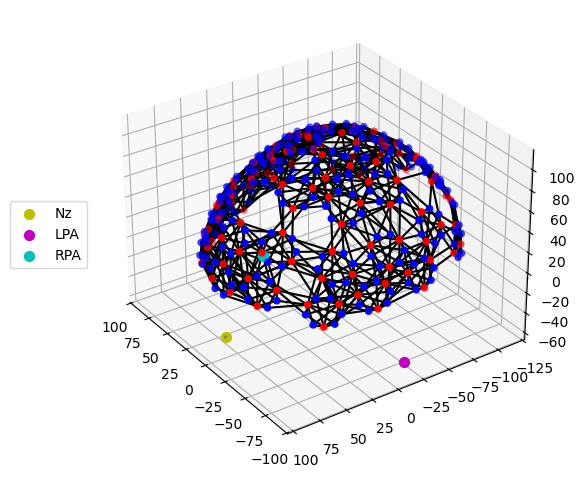
Step 2 — Montage visualisation
Visualising the probe montage on a head surface confirms that the optodes are in anatomically plausible positions and gives an immediate sense of the cortical coverage.
We first plot the raw digitised positions reported in the SNIRF file, then register them to the Colin27 atlas scalp surface. Registration involves two sub-steps:
Landmark normalisation — map vendor-specific landmark labels (e.g.
"Nz","nz","nasion") to a common naming convention so they align with the atlas landmarks.Scalp snapping — rigidly align the digitised positions to the atlas and project each optode onto the nearest point on the scalp mesh.
To learn more about probe registration and co-registration using photogrammetry, see the Photogrammetric Co-Registration Notebook.
[30]:
# Quick 3-D view of the optode positions as stored in the SNIRF file,
# without any registration to a head model.
cedalion.vis.anatomy.plot_montage3D(amp, rec.geo3d)
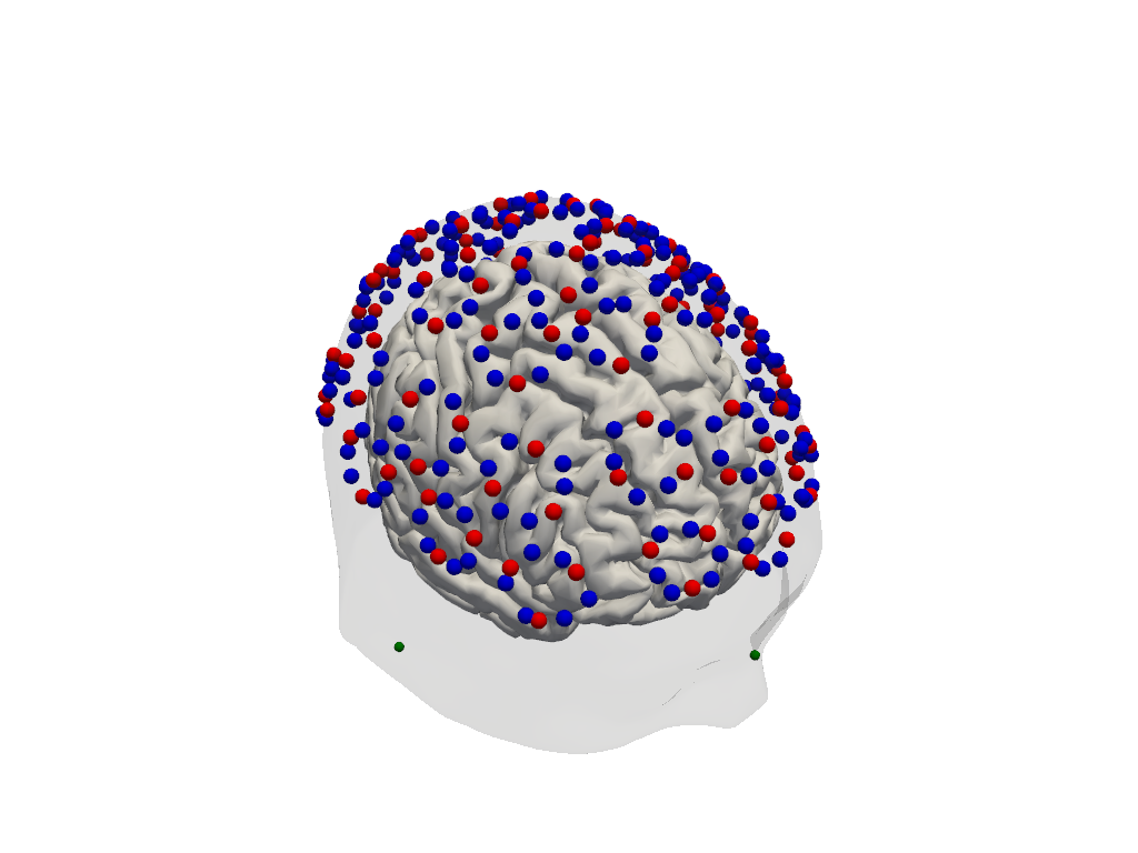
[31]:
# Normalise landmark labels so they match the atlas convention, then
# rigidly align and relax the optode positions onto the Colin27 scalp surface.
geo3d = normalize_landmarks_labels(rec.geo3d)
geo3d_snapped, _ = head_ras.align_and_relax_to_scalp(
    geo3d, rec["amp"], initial_align_mode="trans_rot_isoscale" # only 3 landmarks available
)

# Render the scalp (semi-transparent) and cortex together with the registered optodes.
plotter = pv.Plotter()
vbx.plot_surface(plotter, head_ras.scalp, opacity=0.1)
vbx.plot_surface(plotter, head_ras.brain, color="w")
vbx.plot_labeled_points(plotter, geo3d_snapped)
plotter.show()
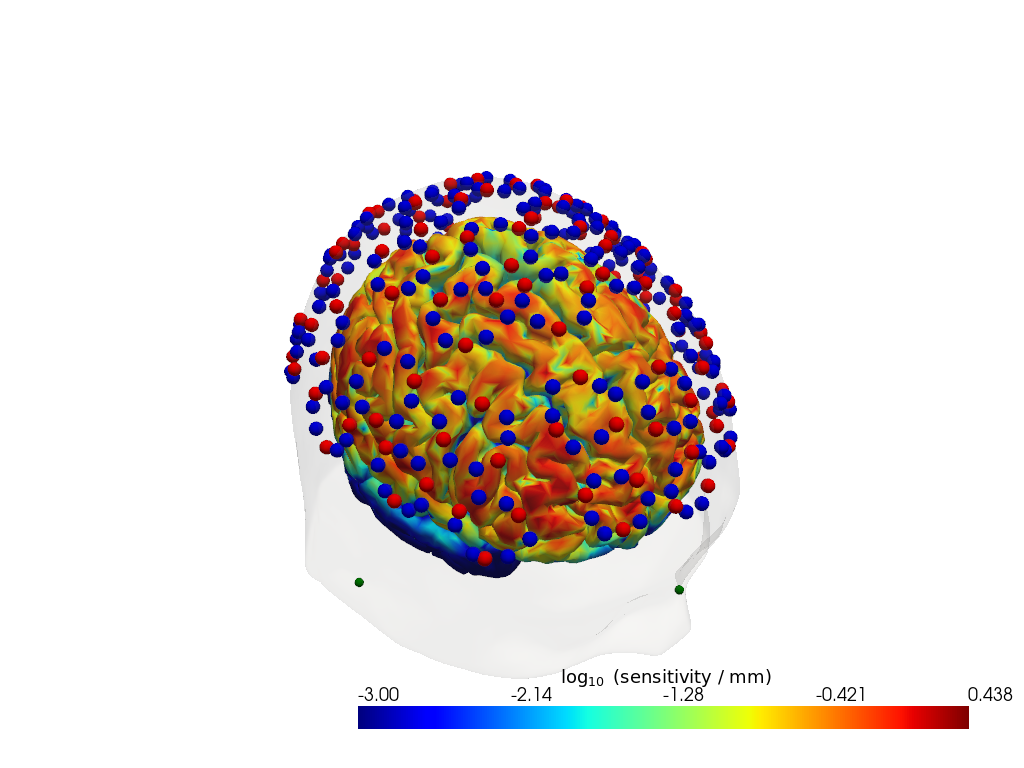
Step 3 — Sensitivity profile
The sensitivity matrix (also called the Jacobian or A matrix) quantifies how much each cortical voxel contributes to each measured channel. Visualising the maximum sensitivity across all channels gives an intuitive map of the cortical area covered by the montage and reveals potential blind spots.
Computing the sensitivity matrix requires running a photon transport simulation (Monte Carlo or FEM), which is computationally expensive. Here we load a pre-computed sensitivity matrix for this dataset. To learn how to compute your own, see the image reconstruction notebook.
[32]:
# Load a pre-computed sensitivity matrix for this dataset at the Colin27 atlas.
Adot = cedalion.data.get_precomputed_sensitivity("kernel_testdataset", "colin27")

# For a spatial overview, take the maximum sensitivity across all channels at 850 nm.
# Restricting to brain vertices avoids scalp contributions dominating the colour scale.
# Log10 is applied because sensitivity varies over several orders of magnitude with depth.
sensitivity = Adot.sel(vertex=Adot.is_brain, wavelength=905).max("channel")

plotter = pv.Plotter()
vbx.plot_surface(plotter, head_ras.scalp, color="w", opacity=0.1)
vbx.plot_surface(plotter, head_ras.brain, color=np.log10(np.clip(sensitivity, 1e-3, 1e1)),  **sensitivity_kwargs)
vbx.plot_labeled_points(plotter, geo3d_snapped)
plotter.show()
Downloading file 'sensitivity_kernel_testdataset_colin27.nc' from 'https://doc.ibs.tu-berlin.de/cedalion/datasets/dev/sensitivity_kernel_testdataset_colin27.nc' to '/home/runner/.cache/cedalion/dev'.
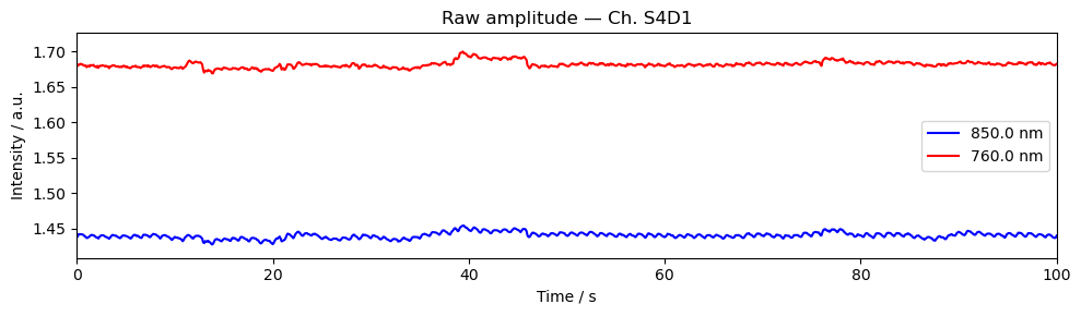
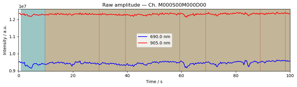
Step 4 — Time series
A quick look at the raw amplitude time series for a single channel confirms that the signal is present and physiologically plausible. Things to look for:
A clear cardiac pulse (~1 Hz oscillation visible in a short window).
No flat sections or sudden jumps that would indicate a saturated or disconnected optode.
Stimulus markers aligned with the expected task timings.
For detailed time series visualisation across many channels — including butterfly plots, quality overlays, and epoch-locked averages — see the Visualization Examples Notebook.
[33]:
ch = amp.channel[0].item()  # pick first channel; replace with a specific channel name if desired

fig, ax = plt.subplots(figsize=(10, 3))
for wl, color in zip(amp.wavelength.values, ["b", "r"]):
    ax.plot(amp.time, amp.sel(channel=ch, wavelength=wl), color=color, label=f"{wl} nm")
ax.set_title(f"Raw amplitude — Ch. {ch}")
ax.set_xlabel("Time / s")
ax.set_ylabel("Intensity / a.u.")
ax.set_xlim(0, 100)
ax.legend()
vbx.plot_stim_markers(ax, rec.stim, y=1)
plt.tight_layout()
plt.show()
References
[34]:
cedalion.bib.dump_to_notebook()
Methods used
| [1] | Holmes1998 | cedalion.data.get_colin27_headmodel_files | Colin J. Holmes, Rick Hoge, Louis Collins, Roger Woods, Arthur W. Toga, and Alan C. Evans. Enhancement of mr images using registration for signal averaging. Journal of Computer Assisted Tomography, 22(2):324–333, March 1998. doi:10.1097/00004728-199803000-00032. |
| [2] | Fischl2012 | cedalion.data.get_colin27_headmodel_files | Bruce Fischl. FreeSurfer. NeuroImage, 62(2):774–781, 2012. doi:10.1016/j.neuroimage.2012.01.021. |
| [3] | Schaefer2018 | cedalion.data.get_colin27_headmodel_files | Alexander Schaefer, Ru Kong, Evan M Gordon, Timothy O Laumann, Xi-Nian Zuo, Avram J Holmes, Simon B Eickhoff, and BT Thomas Yeo. Local-global parcellation of the human cerebral cortex from intrinsic functional connectivity mri. Cerebral cortex, 28(9):3095–3114, 2018. doi:10.1093/cercor/bhx179. |
| [4] | Tucker2022 | cedalion.io.snirf.read_snirf | Stephen Tucker, Jay Dubb, Sreekanth Kura, Alexander von Lühmann, Robert Franke, Jörn M. Horschig, Samuel Powell, Robert Oostenveld, Michael Lührs, Édouard Delaire, Zahra M. Aghajan, Hanseok Yun, Meryem A. Yücel, Qianqian Fang, Theodore J. Huppert, Blaise deB. Frederick, Luca Pollonini, David A. Boas, and Robert Luke. Introduction to the shared near infrared spectroscopy format. Neurophotonics, 10(1):013507, 2022. doi:10.1117/1.NPh.10.1.013507. |
| [5] | Huppert2009 | cedalion.sigproc.quality.snr | Theodore J. Huppert, Solomon G. Diamond, Maria A. Franceschini, and David A. Boas. Homer: a review of time-series analysis methods for near-infrared spectroscopy of the brain. Appl. Opt., 48(10):D280–D298, Apr 2009. doi:https://doi.org/10.1364/AO.48.00D280. |
| [6] | Aasted2015 | cedalion.dot.head_model.TwoSurfaceHeadModel.align_and_relax_to_scalp | Christopher M. Aasted, Meryem A. Yücel, Robert J. Cooper, Jay Dubb, Daisuke Tsuzuki, Lino Becerra, Martin P. Petkov, David Borsook, Ippeita Dan, and David A. Boas. Anatomical guidance for functional near-infrared spectroscopy: AtlasViewer tutorial. Neurophotonics, 2(2):020801, 2015. doi:10.1117/1.NPh.2.2.020801. |
| [7] | Fang2009 | cedalion.data.get_precomputed_sensitivity | Qianqian Fang and David A Boas. Monte carlo simulation of photon migration in 3d turbid media accelerated by graphics processing units. Optics express, 17(22):20178–20190, 2009. doi:10.1364/OE.17.020178. |
| [8] | Yu2018 | cedalion.data.get_precomputed_sensitivity | Leiming Yu, Fanny Nina-Paravecino, David Kaeli, and Qianqian Fang. Scalable and massively parallel monte carlo photon transport simulations for heterogeneous computing platforms. Journal of biomedical optics, 23(1):010504–010504, 2018. doi:10.1117/1.JBO.23.1.010504. |
| [9] | Yan2020 | cedalion.data.get_precomputed_sensitivity | Shijie Yan and Qianqian Fang. Hybrid mesh and voxel based monte carlo algorithm for accurate and efficient photon transport modeling in complex bio-tissues. Biomedical Optics Express, 11(11):6262–6270, 2020. doi:10.1364/BOE.409468. |