Storing estimated HRFs in snirf files
This notebook estimates the HRF in a finger-tapping experiment by blockaveraging and then stores the result in a snirf file.
[1]:
# This cells setups the environment when executed in Google Colab.
try:
    import google.colab
    !curl -s https://raw.githubusercontent.com/ibs-lab/cedalion/dev/scripts/colab_setup.py -o colab_setup.py
    # Select branch with --branch "branch name" (default is "dev")
    %run colab_setup.py
except ImportError:
    pass
[2]:
from pathlib import Path
import tempfile

import matplotlib.pyplot as p
import numpy as np
import xarray as xr
from snirf import Snirf

import cedalion
import cedalion.data
import cedalion.io
import cedalion.nirs

from cedalion import units

xr.set_options(display_max_rows=3, display_values_threshold=50, display_expand_data=False)
np.set_printoptions(precision=4)
Load a finger-tapping dataset
For this demo we load an example finger-tapping recording through cedalion.data.get_fingertapping. The file contains a single NIRS element with one block of raw amplitude data.
[3]:
rec = cedalion.data.get_fingertapping()
[4]:
# Rename events
rec.stim.cd.rename_events( {
    "1.0" : "control",
    "2.0" : "Tapping/Left",
    "3.0" : "Tapping/Right"
})
Calculate concentrations
[5]:
dpf = xr.DataArray([6, 6], dims="wavelength", coords={"wavelength" : rec["amp"].wavelength})
rec["od"] = - np.log( rec["amp"] / rec["amp"].mean("time") )
rec["conc"] = cedalion.nirs.cw.beer_lambert(rec["amp"], rec.geo3d, dpf)
Frequency filtering and splitting into epochs
[6]:
rec["conc_freqfilt"] = rec["conc"].cd.freq_filter(fmin=0.02, fmax=0.5, butter_order=4)


cf_epochs = rec["conc_freqfilt"].cd.to_epochs(
    rec.stim,  # stimulus dataframe
    ["Tapping/Left", "Tapping/Right"],  # select events
    before=5 * units.s,  # seconds before stimulus
    after=20 * units.s,  # seconds after stimulus
)
Blockaveraging to estimate the HRFs
[7]:
# calculate baseline
baseline = cf_epochs.sel(reltime=(cf_epochs.reltime < 0)).mean("reltime")
# subtract baseline
epochs_blcorrected = cf_epochs - baseline

# group trials by trial_type. For each group individually average the epoch dimension
rec["hrf_blockaverage"] = epochs_blcorrected.groupby("trial_type").mean("epoch")

display(rec["hrf_blockaverage"])
<xarray.DataArray (trial_type: 2, chromo: 2, channel: 28, reltime: 198)> Size: 177kB
[µM] -0.05277 -0.05263 -0.05258 -0.05263 ... -0.005955 -0.007018 -0.00833
Coordinates: (3/6)
  * reltime     (reltime) float64 2kB -5.12 -4.992 -4.864 ... 19.84 19.97 20.1
  * chromo      (chromo) <U3 24B 'HbO' 'HbR'
    ...          ...
* trial_type (trial_type) object 16B 'Tapping/Left' 'Tapping/Right'Store HRFs
[8]:
tmpdir = tempfile.TemporaryDirectory()
snirf_fname = str(Path(tmpdir.name) / "test.snirf")
[9]:
cedalion.io.snirf.write_snirf(snirf_fname, rec)
Inspect snirf file
[10]:
s = Snirf(snirf_fname)
[11]:
display(s.nirs)
display(s.nirs[0].data)
<iterable of 1 <class 'snirf.pysnirf2.NirsElement'>>
<iterable of 5 <class 'snirf.pysnirf2.DataElement'>>
Stim DataFrame
[12]:
display(s.nirs[0].stim)
<iterable of 4 <class 'snirf.pysnirf2.StimElement'>>
[13]:
cedalion.io.snirf.stim_to_dataframe(s.nirs[0].stim)
[13]:
| onset | duration | value | trial_type | |
|---|---|---|---|---|
| 0 | 61.824 | 5.0 | 1.0 | control |
| 1 | 87.296 | 5.0 | 1.0 | control |
| 2 | 181.504 | 5.0 | 1.0 | control |
| 3 | 275.712 | 5.0 | 1.0 | control |
| 4 | 544.640 | 5.0 | 1.0 | control |
| ... | ... | ... | ... | ... |
| 87 | 2234.112 | 5.0 | 1.0 | Tapping/Right |
| 88 | 2334.848 | 5.0 | 1.0 | Tapping/Right |
| 89 | 2362.240 | 5.0 | 1.0 | Tapping/Right |
| 90 | 2677.504 | 5.0 | 1.0 | Tapping/Right |
| 91 | 2908.032 | 5.0 | 1.0 | Tapping/Right |
92 rows × 4 columns
MeasurementList DataFrame
[14]:
for i_data in range(len(s.nirs[0].data)):
    df_ml = cedalion.io.snirf.measurement_list_to_dataframe(
        s.nirs[0].data[i_data].measurementList, drop_none=True
    )
    display(df_ml.head(3))
    display(df_ml.tail(3))
| sourceIndex | detectorIndex | wavelengthIndex | dataType | dataUnit | |
|---|---|---|---|---|---|
| 0 | 1 | 1 | 1 | 1 | volt |
| 1 | 1 | 1 | 2 | 1 | volt |
| 2 | 1 | 2 | 1 | 1 | volt |
| sourceIndex | detectorIndex | wavelengthIndex | dataType | dataUnit | |
|---|---|---|---|---|---|
| 53 | 8 | 8 | 2 | 1 | volt |
| 54 | 8 | 16 | 1 | 1 | volt |
| 55 | 8 | 16 | 2 | 1 | volt |
| sourceIndex | detectorIndex | wavelengthIndex | dataType | dataUnit | dataTypeLabel | |
|---|---|---|---|---|---|---|
| 0 | 1 | 1 | 1 | 99999 | dimensionless | dOD |
| 1 | 1 | 1 | 2 | 99999 | dimensionless | dOD |
| 2 | 1 | 2 | 1 | 99999 | dimensionless | dOD |
| sourceIndex | detectorIndex | wavelengthIndex | dataType | dataUnit | dataTypeLabel | |
|---|---|---|---|---|---|---|
| 53 | 8 | 8 | 2 | 99999 | dimensionless | dOD |
| 54 | 8 | 16 | 1 | 99999 | dimensionless | dOD |
| 55 | 8 | 16 | 2 | 99999 | dimensionless | dOD |
| sourceIndex | detectorIndex | dataType | dataUnit | dataTypeLabel | |
|---|---|---|---|---|---|
| 0 | 1 | 1 | 99999 | micromolar | HbO |
| 1 | 1 | 1 | 99999 | micromolar | HbR |
| 2 | 1 | 2 | 99999 | micromolar | HbO |
| sourceIndex | detectorIndex | dataType | dataUnit | dataTypeLabel | |
|---|---|---|---|---|---|
| 53 | 8 | 8 | 99999 | micromolar | HbR |
| 54 | 8 | 16 | 99999 | micromolar | HbO |
| 55 | 8 | 16 | 99999 | micromolar | HbR |
| sourceIndex | detectorIndex | dataType | dataUnit | dataTypeLabel | |
|---|---|---|---|---|---|
| 0 | 1 | 1 | 99999 | micromolar | HbO |
| 1 | 1 | 1 | 99999 | micromolar | HbR |
| 2 | 1 | 2 | 99999 | micromolar | HbO |
| sourceIndex | detectorIndex | dataType | dataUnit | dataTypeLabel | |
|---|---|---|---|---|---|
| 53 | 8 | 8 | 99999 | micromolar | HbR |
| 54 | 8 | 16 | 99999 | micromolar | HbO |
| 55 | 8 | 16 | 99999 | micromolar | HbR |
| sourceIndex | detectorIndex | dataType | dataUnit | dataTypeLabel | dataTypeIndex | |
|---|---|---|---|---|---|---|
| 0 | 1 | 1 | 99999 | micromolar | HRF HbO | 3 |
| 1 | 1 | 1 | 99999 | micromolar | HRF HbR | 3 |
| 2 | 1 | 2 | 99999 | micromolar | HRF HbO | 3 |
| sourceIndex | detectorIndex | dataType | dataUnit | dataTypeLabel | dataTypeIndex | |
|---|---|---|---|---|---|---|
| 109 | 8 | 8 | 99999 | micromolar | HRF HbR | 4 |
| 110 | 8 | 16 | 99999 | micromolar | HRF HbO | 4 |
| 111 | 8 | 16 | 99999 | micromolar | HRF HbR | 4 |
[15]:
s.close()
Read HRFs from snirf file
Note: read_snirf names the time dimension time whereas in blockaverage it was called reltime. Need to agree on a convention.
[16]:
hrf_recs = cedalion.io.read_snirf(snirf_fname)
display(hrf_recs)
[<Recording | timeseries: ['amp', 'od', 'conc', 'conc_02', 'hrf_conc'], masks: [], stim: ['control', '15.0', 'Tapping/Left', 'Tapping/Right'], aux_ts: [], aux_obj: []>]
[17]:
# the name of the stored blockaverages derives from the datatype (HRF) and the type of data (concentration)
read_blockaverage = hrf_recs[0]["hrf_conc"]
display(read_blockaverage)
<xarray.DataArray (channel: 28, chromo: 2, trial_type: 2, time: 198)> Size: 177kB
[µM] -0.05277 -0.05263 -0.05258 -0.05263 ... -0.005955 -0.007018 -0.00833
Coordinates: (3/7)
  * time        (time) float64 2kB -5.12 -4.992 -4.864 ... 19.84 19.97 20.1
    samples     (time) int64 2kB 0 1 2 3 4 5 6 7 ... 191 192 193 194 195 196 197
    ...          ...
  * trial_type  (trial_type) <U13 104B 'Tapping/Left' 'Tapping/Right'
Attributes:
data_type_group: processed HRF concentrationsAssert that the written and read HRFs are identical.
[18]:
assert (read_blockaverage.rename({"time" : "reltime"}) == rec["hrf_blockaverage"]).all()
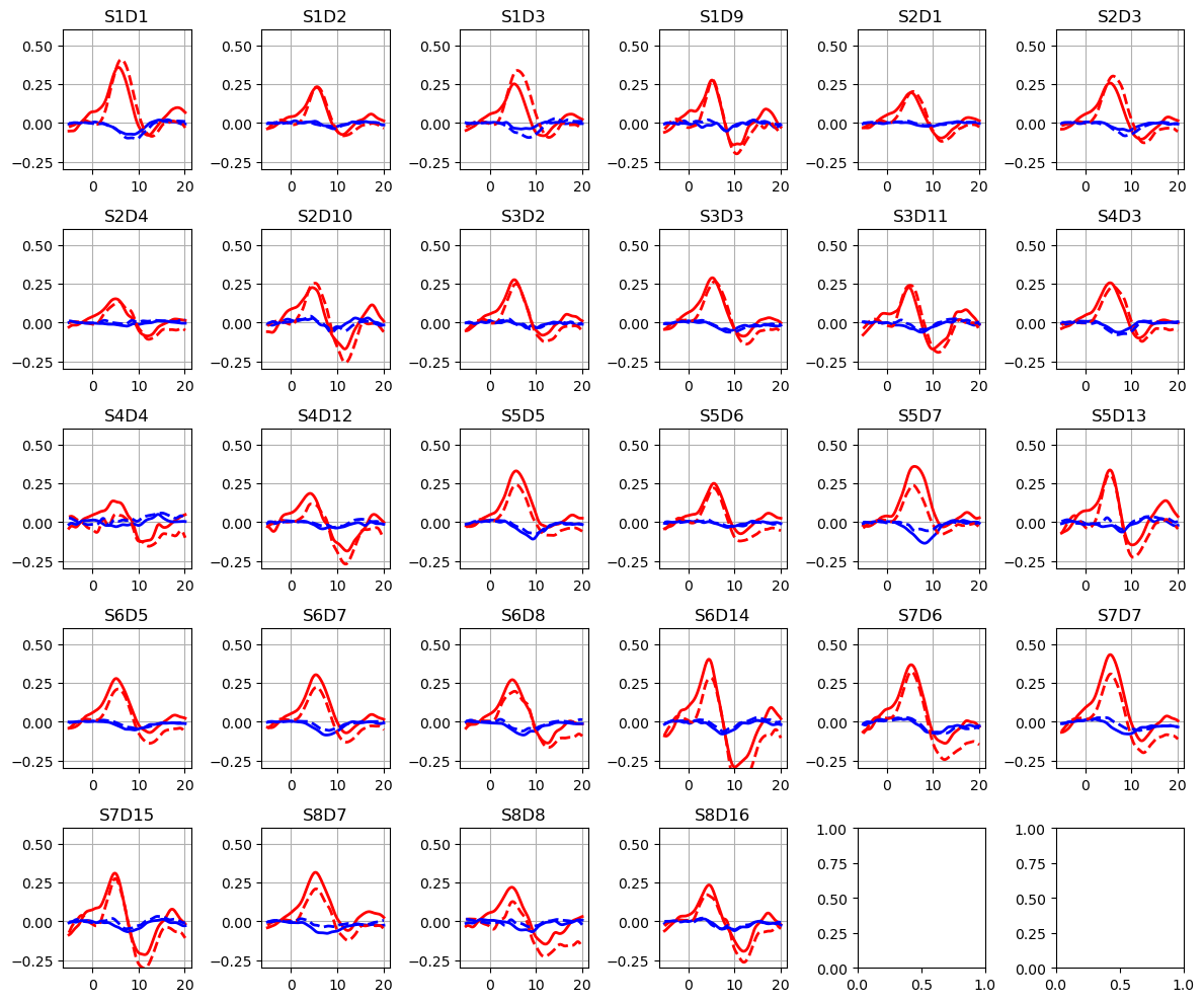
Plot the HRFs
[19]:
ba = read_blockaverage

f,ax = p.subplots(5,6, figsize=(12,10))
ax = ax.flatten()
for i_ch, ch in enumerate(ba.channel.values):
    for ls, trial_type in zip(["-", "--"], ba.trial_type):
        ax[i_ch].plot(ba.time, ba.sel(chromo="HbO", trial_type=trial_type, channel=ch), "r", lw=2, ls=ls)
        ax[i_ch].plot(ba.time, ba.sel(chromo="HbR", trial_type=trial_type, channel=ch), "b", lw=2, ls=ls)
    ax[i_ch].grid(1)
    ax[i_ch].set_title(ch)
    ax[i_ch].set_ylim(-.3, .6)

p.tight_layout()
Tidy up
[20]:
del tmpdir
References
[21]:
cedalion.bib.dump_to_notebook()
Methods used
| [1] | Luke2021 | cedalion.data.get_fingertapping | Robert Luke and David McAlpine. fNIRS Finger Tapping Data in BIDS Format. September 2021. doi:10.5281/zenodo.5529797. |
| [2] | Tucker2022 | cedalion.io.snirf.read_snirf | Stephen Tucker, Jay Dubb, Sreekanth Kura, Alexander von Lühmann, Robert Franke, Jörn M. Horschig, Samuel Powell, Robert Oostenveld, Michael Lührs, Édouard Delaire, Zahra M. Aghajan, Hanseok Yun, Meryem A. Yücel, Qianqian Fang, Theodore J. Huppert, Blaise deB. Frederick, Luca Pollonini, David A. Boas, and Robert Luke. Introduction to the shared near infrared spectroscopy format. Neurophotonics, 10(1):013507, 2022. doi:10.1117/1.NPh.10.1.013507. |
| [3] | Delpy1988 | cedalion.nirs.cw.beer_lambert, cedalion.nirs.cw.int2od, cedalion.nirs.cw.od2conc | D. T. Delpy, M. Cope, P. van der Zee, S. Arridge, S. Wray, and J. Wyatt. Estimation of optical pathlength through tissue from direct time of flight measurement. Physics in Medicine and Biology, 33(12):1433–1442, 1988. doi:10.1088/0031-9155/33/12/008. |
| [4] | Villringer1997 | cedalion.nirs.cw.beer_lambert, cedalion.nirs.cw.int2od, cedalion.nirs.cw.od2conc | Arno Villringer and Britton Chance. Non-invasive optical spectroscopy and imaging of human brain function. Trends in Neurosciences, 20(10):435–442, 1997. doi:10.1016/S0166-2236(97)01132-6. |
| [5] | Prahl1998 | cedalion.nirs.common.get_extinction_coefficients | Scott A. Prahl. Optical absorption of hemoglobin. Oregon Medical Laser Center, online resource, 1998. URL: https://omlc.org/spectra/hemoglobin/. |