Statsmodels Methods Overview
[1]:
# This cells setups the environment when executed in Google Colab.
try:
    import google.colab
    !curl -s https://raw.githubusercontent.com/ibs-lab/cedalion/dev/scripts/colab_setup.py -o colab_setup.py
    # Select branch with --branch "branch name" (default is "dev")
    %run colab_setup.py
except ImportError:
    pass
Cedalion uses statsmodels for its GLM fitting functionality, and this notebook gives an overview of some common statsmodels methods. The glm.fit function returns an xr.DataArray of statsmodels RegressionResults objects with dimensions (channel, chromo). Any RegressionResults method can be called on this DataArray using the .sm accessor. A full list of available methods and attribute can be found in the statsmodels documentation.
In this notebook, we’ll assume that we have already loaded our data and set up the GLM. See the other GLM notebooks for details on setup.
We’ll start by fitting the GLM and displaying the resulting object.
[3]:
results = glm.fit(ts_long, dms)
display(results)
 67%|██████▋   | 2/3 [00:00<00:00, 154.92it/s]
 67%|██████▋   | 2/3 [00:00<00:00, 81.86it/s]
 50%|█████     | 1/2 [00:00<00:00, 85.44it/s]
 50%|█████     | 1/2 [00:00<00:00, 84.68it/s]
 67%|██████▋   | 2/3 [00:00<00:00, 164.65it/s]
 67%|██████▋   | 2/3 [00:00<00:00, 162.43it/s]
 50%|█████     | 1/2 [00:00<00:00, 85.58it/s]
 50%|█████     | 1/2 [00:00<00:00, 86.43it/s]
 67%|██████▋   | 2/3 [00:00<00:00, 162.47it/s]
 67%|██████▋   | 2/3 [00:00<00:00, 160.58it/s]
 50%|█████     | 1/2 [00:00<00:00, 84.77it/s]
 50%|█████     | 1/2 [00:00<00:00, 85.45it/s]
 67%|██████▋   | 2/3 [00:00<00:00, 84.27it/s]
 67%|██████▋   | 2/3 [00:00<00:00, 90.31it/s]
 50%|█████     | 1/2 [00:00<00:00, 87.24it/s]
 50%|█████     | 1/2 [00:00<00:00, 83.80it/s]
<xarray.DataArray (channel: 20, chromo: 2)> Size: 320B
<statsmodels.regression.linear_model.RegressionResultsWrapper object at 0x7fe...
Coordinates:
  * chromo    (chromo) <U3 24B 'HbO' 'HbR'
  * channel   (channel) object 160B 'S1D1' 'S1D2' 'S1D3' ... 'S8D7' 'S8D8'
    source    (channel) object 160B 'S1' 'S1' 'S1' 'S2' ... 'S7' 'S7' 'S8' 'S8'
    detector  (channel) object 160B 'D1' 'D2' 'D3' 'D1' ... 'D6' 'D7' 'D7' 'D8'
Attributes:
description: OLS model via statsmodels.regressionThe results object is a DataArray of statsmodels RegressionResults: one for each channel/chromophore. In order to call a method on our results object, we just use the accessor .sm, followed by the RegressionResults method. Cedalion handles calling the method on each individual RegressionResults object in the results DataArray, and returns the outputs in a new DataArray with the
appropriate dimensions. This allows us to get information on all channels simply and concisely.
Beta Coefficients (params)
First, we’ll retreive the coefficients of the GLM fit.
[4]:
results.sm.params
[4]:
<xarray.DataArray (channel: 20, chromo: 2, regressor: 4)> Size: 1kB
-5.405e-05 0.006065 0.007626 0.7729 ... -0.00051 -0.0006538 -0.0007396 -0.03845
Coordinates:
  * regressor  (regressor) object 32B 'HRF control' ... 'short'
  * chromo     (chromo) <U3 24B 'HbO' 'HbR'
  * channel    (channel) object 160B 'S1D1' 'S1D2' 'S1D3' ... 'S8D7' 'S8D8'
    source     (channel) object 160B 'S1' 'S1' 'S1' 'S2' ... 'S7' 'S7' 'S8' 'S8'
    detector   (channel) object 160B 'D1' 'D2' 'D3' 'D1' ... 'D6' 'D7' 'D7' 'D8'
Attributes:
description: OLS model via statsmodels.regressionStandard Error
The method bse returns the standard errors of the parameter estimates
[5]:
results.sm.bse
[5]:
<xarray.DataArray (channel: 20, chromo: 2, regressor: 4)> Size: 1kB
0.000188 0.0001896 0.0001902 0.005514 ... 0.0001074 0.0001074 0.0001075 0.006336
Coordinates:
  * regressor  (regressor) object 32B 'HRF control' ... 'short'
  * chromo     (chromo) <U3 24B 'HbO' 'HbR'
  * channel    (channel) object 160B 'S1D1' 'S1D2' 'S1D3' ... 'S8D7' 'S8D8'
    source     (channel) object 160B 'S1' 'S1' 'S1' 'S2' ... 'S7' 'S7' 'S8' 'S8'
    detector   (channel) object 160B 'D1' 'D2' 'D3' 'D1' ... 'D6' 'D7' 'D7' 'D8'
Attributes:
description: OLS model via statsmodels.regressionConfidence Intervals (conf_int)
The method conf_int calculates the confidence interval of the fitted parameters. We can specify the alpha level for the confidence interval (default 5%).
In the output, the index conf_int marks the low (conf_int=0) and high (conf_int=1) endpoints of the confidence interval.
[6]:
results.sm.conf_int(alpha=0.05)
[6]:
<xarray.DataArray (channel: 20, chromo: 2, regressor: 4, conf_int: 2)> Size: 3kB
-0.0004225 0.0003144 0.005693 0.006436 ... -0.000529 -0.05087 -0.02603
Coordinates:
  * regressor  (regressor) object 32B 'HRF control' ... 'short'
  * conf_int   (conf_int) int64 16B 0 1
  * chromo     (chromo) <U3 24B 'HbO' 'HbR'
  * channel    (channel) object 160B 'S1D1' 'S1D2' 'S1D3' ... 'S8D7' 'S8D8'
    source     (channel) object 160B 'S1' 'S1' 'S1' 'S2' ... 'S7' 'S7' 'S8' 'S8'
    detector   (channel) object 160B 'D1' 'D2' 'D3' 'D1' ... 'D6' 'D7' 'D7' 'D8'
Attributes:
description: OLS model via statsmodels.regressionCovariance and Variance
The method cov_params computes the covariance matrix. Note that we can recover the variances from the diagonal elements of the matrix.
[7]:
results.sm.cov_params()
[7]:
<xarray.DataArray (channel: 20, chromo: 2, regressor_r: 4, regressor_c: 4)> Size: 5kB
3.534e-08 -6.447e-11 -7.449e-11 1.432e-08 ... 8.799e-09 2.807e-08 4.014e-05
Coordinates:
  * regressor_r  (regressor_r) object 32B 'HRF control' ... 'short'
  * regressor_c  (regressor_c) object 32B 'HRF control' ... 'short'
  * chromo       (chromo) <U3 24B 'HbO' 'HbR'
  * channel      (channel) object 160B 'S1D1' 'S1D2' 'S1D3' ... 'S8D7' 'S8D8'
    source       (channel) object 160B 'S1' 'S1' 'S1' 'S2' ... 'S7' 'S8' 'S8'
    detector     (channel) object 160B 'D1' 'D2' 'D3' 'D1' ... 'D7' 'D7' 'D8'
Attributes: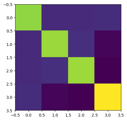
description: OLS model via statsmodels.regressionHere we visualize the covariance matrix for a single regressor:
[8]:
p.imshow(results.sm.cov_params()[0,0,:,:]);
The convenience function sm.regressor_variances computes the variances of the regressors, i.e. the diagonal elements of the covariance matrices.
[9]:
# returns diagonal elements of the cov matrices
results.sm.regressor_variances()
[9]:
<xarray.DataArray (channel: 20, chromo: 2, regressor: 4)> Size: 1kB
3.534e-08 3.595e-08 3.616e-08 3.04e-05 ... 1.153e-08 1.155e-08 4.014e-05
Coordinates:
  * regressor  (regressor) object 32B 'HRF control' ... 'short'
  * chromo     (chromo) <U3 24B 'HbO' 'HbR'
  * channel    (channel) object 160B 'S1D1' 'S1D2' 'S1D3' ... 'S8D7' 'S8D8'
    source     (channel) object 160B 'S1' 'S1' 'S1' 'S2' ... 'S7' 'S7' 'S8' 'S8'
    detector   (channel) object 160B 'D1' 'D2' 'D3' 'D1' ... 'D6' 'D7' 'D7' 'D8'
Attributes:
description: OLS model via statsmodels.regressionStatistical Tests - T-values, P-values
Statsmodels also has sophisticated functionality for performing statistical tests on regression results.
The method t-values simply returns the t-statistic for each coefficient.
[10]:
results.sm.tvalues
[10]:
<xarray.DataArray (channel: 20, chromo: 2, regressor: 4)> Size: 1kB
-0.2875 31.98 40.1 140.2 -1.327 -17.83 ... 97.04 -4.749 -6.089 -6.882 -6.069
Coordinates:
  * regressor  (regressor) object 32B 'HRF control' ... 'short'
  * chromo     (chromo) <U3 24B 'HbO' 'HbR'
  * channel    (channel) object 160B 'S1D1' 'S1D2' 'S1D3' ... 'S8D7' 'S8D8'
    source     (channel) object 160B 'S1' 'S1' 'S1' 'S2' ... 'S7' 'S7' 'S8' 'S8'
    detector   (channel) object 160B 'D1' 'D2' 'D3' 'D1' ... 'D6' 'D7' 'D7' 'D8'
Attributes:
description: OLS model via statsmodels.regressionThe method t-test allows for general linear hypothesis tests.
We can specify contrasts either by passing an r-matrix or through strings. See the patsy documentation for details on specifying linear contrasts using strings.
The method returns an array of statsmodel ContrastResult objects.
[11]:
# Specifying hypotheses for t-test as string
hypotheses = "HRF Tapping/Left = HRF control, HRF Tapping/Right = HRF control"

contrast_results = results.sm.t_test(hypotheses)
display(contrast_results)
<xarray.DataArray (channel: 20, chromo: 2)> Size: 320B
                             Test for Constraints                            ...
Coordinates:
  * chromo    (chromo) <U3 24B 'HbO' 'HbR'
  * channel   (channel) object 160B 'S1D1' 'S1D2' 'S1D3' ... 'S8D7' 'S8D8'
    source    (channel) object 160B 'S1' 'S1' 'S1' 'S2' ... 'S7' 'S7' 'S8' 'S8'
    detector  (channel) object 160B 'D1' 'D2' 'D3' 'D1' ... 'D6' 'D7' 'D7' 'D8'
Attributes:
description: OLS model via statsmodels.regressionWe can use the .sm accessor on the resulting DataArray of ContrastResult objects, just like we did before with the RegressionResult arrays.
The convenience functions sm.tvalues() and sm.pvalues() return the t- and p-values of the contrast, respectively.
The sm.map method works analogously to the map function in python, applying a given function to each cell of the DataArray.
Below, we extract the t-values of the contrast using first the map method and then the convenience function.
[12]:
# Extracting t-values from the contrast results
display(contrast_results.sm.map(lambda i : i.tvalue, name="hypothesis"))

display(contrast_results.sm.t_values())
<xarray.DataArray (channel: 20, chromo: 2, hypothesis: 2)> Size: 640B
22.89 28.69 -11.67 -14.53 18.91 20.18 ... -12.03 -3.51 11.8 9.7 -0.947 -1.511
Coordinates:
  * chromo    (chromo) <U3 24B 'HbO' 'HbR'
  * channel   (channel) object 160B 'S1D1' 'S1D2' 'S1D3' ... 'S8D7' 'S8D8'
    source    (channel) object 160B 'S1' 'S1' 'S1' 'S2' ... 'S7' 'S7' 'S8' 'S8'
    detector  (channel) object 160B 'D1' 'D2' 'D3' 'D1' ... 'D6' 'D7' 'D7' 'D8'
Dimensions without coordinates: hypothesis
Attributes:
description: OLS model via statsmodels.regression<xarray.DataArray (channel: 20, chromo: 2, hypothesis: 2)> Size: 640B
22.89 28.69 -11.67 -14.53 18.91 20.18 ... -12.03 -3.51 11.8 9.7 -0.947 -1.511
Coordinates:
* chromo (chromo) <U3 24B 'HbO' 'HbR'
* channel (channel) object 160B 'S1D1' 'S1D2' 'S1D3' ... 'S8D7' 'S8D8'
source (channel) object 160B 'S1' 'S1' 'S1' 'S2' ... 'S7' 'S7' 'S8' 'S8'
detector (channel) object 160B 'D1' 'D2' 'D3' 'D1' ... 'D6' 'D7' 'D7' 'D8'
Dimensions without coordinates: hypothesis
Attributes:
description: OLS model via statsmodels.regression[13]:
# Extracting p-values from the contrast results
display(contrast_results.sm.p_values())
<xarray.DataArray (channel: 20, chromo: 2, hypothesis: 2)> Size: 640B
9.929e-115 6.125e-178 2.164e-31 1.18e-47 ... 5.073e-32 3.313e-22 0.3436 0.1307
Coordinates:
  * chromo    (chromo) <U3 24B 'HbO' 'HbR'
  * channel   (channel) object 160B 'S1D1' 'S1D2' 'S1D3' ... 'S8D7' 'S8D8'
    source    (channel) object 160B 'S1' 'S1' 'S1' 'S2' ... 'S7' 'S7' 'S8' 'S8'
    detector  (channel) object 160B 'D1' 'D2' 'D3' 'D1' ... 'D6' 'D7' 'D7' 'D8'
Dimensions without coordinates: hypothesis
Attributes:
description: OLS model via statsmodels.regressionPlotting Uncertainty Bands
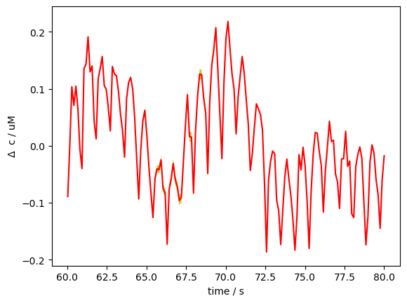
In this section, we explore a technique, still in development, for visualizing uncertainty in a GLM with many regressors. This method visualizes the uncertainty in a GLM fit by drawing multiple samples of the beta coefficients from their estimated covariance (via multivariate normal sampling). It then uses these sampled betas to generate predicted time courses, and plots the mean prediction with a shaded band representing ±3 standard deviations across samples, thus capturing the variability due to model uncertainty. The band is quite narrow because uncertainty is low in this toy example.
FIXME: Band even smaller than before?
[14]:
# Sample betas

betas = results.sm.params
cov = results.sm.cov_params()

sampled_betas = xr.zeros_like(betas).expand_dims({"sample" : 100}, axis=-1).copy()
for i_ch in range(sampled_betas.shape[0]):
    for i_cr in range(sampled_betas.shape[1]):
        sampled_betas[i_ch, i_cr, :, :] = np.random.multivariate_normal(
            betas[i_ch, i_cr, :],
            cov[i_ch, i_cr, :, :],
            size=100,
        ).T

display(sampled_betas)
<xarray.DataArray (channel: 20, chromo: 2, regressor: 4, sample: 100)> Size: 128kB
-0.0001672 -2.997e-05 -0.0003786 -0.0002055 ... -0.03152 -0.03368 -0.02647
Coordinates:
  * regressor  (regressor) object 32B 'HRF control' ... 'short'
  * chromo     (chromo) <U3 24B 'HbO' 'HbR'
  * channel    (channel) object 160B 'S1D1' 'S1D2' 'S1D3' ... 'S8D7' 'S8D8'
    source     (channel) object 160B 'S1' 'S1' 'S1' 'S2' ... 'S7' 'S7' 'S8' 'S8'
    detector   (channel) object 160B 'D1' 'D2' 'D3' 'D1' ... 'D6' 'D7' 'D7' 'D8'
Dimensions without coordinates: sample
Attributes:
description: OLS model via statsmodels.regression[15]:
# Predicting the time series using the sampled betas
pred = glm.predict(ts_long, sampled_betas, dms)
display(pred)
<xarray.DataArray (time: 23239, channel: 20, chromo: 2, sample: 100)> Size: 744MB
-0.0935 -0.09623 -0.09503 -0.09557 ... 8.304e-05 6.616e-05 7.07e-05 5.557e-05
Coordinates:
  * time           (time) float64 186kB 0.0 0.128 0.256 ... 2.974e+03 2.974e+03
  * chromo         (chromo) <U3 24B 'HbO' 'HbR'
    samples        (time) int64 186kB 0 1 2 3 4 ... 23235 23236 23237 23238
  * channel        (channel) object 160B 'S1D1' 'S1D2' 'S1D3' ... 'S8D7' 'S8D8'
    short_channel  (channel) object 160B 'S1D9' 'S1D9' ... 'S8D16' 'S8D16'
    comp_group     (channel) int64 160B 0 0 0 1 1 1 2 2 3 3 4 4 4 5 5 5 6 6 7 7
    source         (channel) object 160B 'S1' 'S1' 'S1' 'S2' ... 'S7' 'S8' 'S8'
    detector       (channel) object 160B 'D1' 'D2' 'D3' 'D1' ... 'D7' 'D7' 'D8'
Dimensions without coordinates: sample[16]:
# Plot a band between mean-3*std and mean+3*std
# We select a 20 second window for better visualization
pred_mean = pred.mean("sample")
pred_std = pred.std("sample")

mm = pred_mean.loc[slice(60,80), "S5D5", "HbO"]
ss = pred_std.loc[slice(60,80), "S5D5", "HbO"]

p.plot(mm.time, mm, c="r")
p.fill_between(mm.time, mm-3*ss, mm+3*ss, fc="y", alpha=.8)

p.xlabel("time / s")
p.ylabel(r"$\Delta$  c / uM");
References
[17]:
cedalion.bib.dump_to_notebook()
Methods used
| [1] | Luke2021 | cedalion.data.get_fingertapping | Robert Luke and David McAlpine. fNIRS Finger Tapping Data in BIDS Format. September 2021. doi:10.5281/zenodo.5529797. |
| [2] | Tucker2022 | cedalion.io.snirf.read_snirf | Stephen Tucker, Jay Dubb, Sreekanth Kura, Alexander von Lühmann, Robert Franke, Jörn M. Horschig, Samuel Powell, Robert Oostenveld, Michael Lührs, Édouard Delaire, Zahra M. Aghajan, Hanseok Yun, Meryem A. Yücel, Qianqian Fang, Theodore J. Huppert, Blaise deB. Frederick, Luca Pollonini, David A. Boas, and Robert Luke. Introduction to the shared near infrared spectroscopy format. Neurophotonics, 10(1):013507, 2022. doi:10.1117/1.NPh.10.1.013507. |
| [3] | Delpy1988 | cedalion.nirs.cw.int2od, cedalion.nirs.cw.od2conc | D. T. Delpy, M. Cope, P. van der Zee, S. Arridge, S. Wray, and J. Wyatt. Estimation of optical pathlength through tissue from direct time of flight measurement. Physics in Medicine and Biology, 33(12):1433–1442, 1988. doi:10.1088/0031-9155/33/12/008. |
| [4] | Villringer1997 | cedalion.nirs.cw.int2od, cedalion.nirs.cw.od2conc | Arno Villringer and Britton Chance. Non-invasive optical spectroscopy and imaging of human brain function. Trends in Neurosciences, 20(10):435–442, 1997. doi:10.1016/S0166-2236(97)01132-6. |
| [5] | Prahl1998 | cedalion.nirs.common.get_extinction_coefficients | Scott A. Prahl. Optical absorption of hemoglobin. Oregon Medical Laser Center, online resource, 1998. URL: https://omlc.org/spectra/hemoglobin/. |
| [6] | Strangman2002 | cedalion.models.glm.basis_functions.Gamma.__call__ | Gary Strangman, Joseph P. Culver, John H. Thompson, and David A. Boas. A quantitative comparison of simultaneous BOLD fMRI and NIRS recordings during functional brain activation. NeuroImage, 17(2):719–731, 2002. doi:10.1006/nimg.2002.1227. |
| [7] | Huppert2009 | cedalion.models.glm.design_matrix.closest_short_channel_regressor | Theodore J. Huppert, Solomon G. Diamond, Maria A. Franceschini, and David A. Boas. Homer: a review of time-series analysis methods for near-infrared spectroscopy of the brain. Appl. Opt., 48(10):D280–D298, Apr 2009. doi:https://doi.org/10.1364/AO.48.00D280. |
| [8] | Barker2013 | cedalion.models.glm.solve.fit | Jeffrey W. Barker, Ardalan Aarabi, and Theodore J. Huppert. Autoregressive model based algorithm for correcting motion and serially correlated errors in fnirs. Biomed. Opt. Express, 4(8):1366–1379, Aug 2013. doi:10.1364/BOE.4.001366. |