Data Structures and I/O
[1]:
# This cells setups the environment when executed in Google Colab.
try:
    import google.colab
    !curl -s https://raw.githubusercontent.com/ibs-lab/cedalion/dev/scripts/colab_setup.py -o colab_setup.py
    # Select branch with --branch "branch name" (default is "dev")
    %run colab_setup.py
except ImportError:
    pass
[2]:
import numpy as np
import pandas as pd
import xarray as xr
import tempfile
from pathlib import Path

import cedalion
import cedalion.io
import cedalion.data
import cedalion.nirs
import cedalion.xrutils as xrutils

pd.set_option('display.max_rows', 10)
xr.set_options(display_expand_data=False);
[3]:
# helper function
def calc_concentratoin(rec):
    od = cedalion.nirs.cw.int2od(rec["amp"])
    dpf = xr.DataArray([6, 6], dims="wavelength", coords={"wavelength" : od.wavelength})
    return cedalion.nirs.cw.od2conc(od, rec.geo3d, dpf)
Reading Snirf Files
Snirf files can be loaded with the cedalion.io.read_snirf method. This returns a list of cedalion.dataclasses.Recording objects. The
[4]:
path_to_snirf_file = cedalion.data.get_fingertapping_snirf_path()

recordings = cedalion.io.read_snirf(path_to_snirf_file)

display(path_to_snirf_file)
display(recordings)
display(len(recordings))
PosixPath('/home/runner/.cache/cedalion/dev/fingertapping.zip.unzip/fingertapping/sub-01_task-tapping_nirs.snirf')
[<Recording | timeseries: ['amp'], masks: [], stim: ['1.0', '15.0', '2.0', '3.0'], aux_ts: [], aux_obj: []>]
1
Accessing example datasets
Example datasets are accessible through functions in cedalion.data. These take care of downloading, caching and updating the data files. Often they also already load the data.
[5]:
rec = cedalion.data.get_fingertapping()
display(rec)
<Recording | timeseries: ['amp'], masks: [], stim: ['1.0', '15.0', '2.0', '3.0'], aux_ts: [], aux_obj: []>
Recording containers
The class cedalion.dataclasses.Recording is Cedalion’s main data container to carry related data objects through the program. It can store time series, masks, auxiliary timeseries, probe, headmodel and stimulus information as well as meta data about the recording. It has the following properties:
field |
description |
|---|---|
timeseries |
a dictionary of timeseries objects |
masks |
a dictionary of masks that flag time points as good or bad |
geo3d |
3D probe geometry |
geo2d |
2D probe geometry |
stim |
dataframe with stimulus information |
aux_ts |
dictionary of auxiliary time series objects |
aux_obj |
dictionary for any other auxiliary objects |
head_model |
voxel image, cortex and scalp surfaces |
meta_data |
dictionary for meta data |
container is very similar to the layout of a snirf file
Recordingmaps mainly to nirs groupstimeseries objects map to data elements
Dictionaries in Recording
dictionaries are key value stores
maintain order in which values are added -> facilitate workflows
the user differentiates time series by name.
names are free to choose but there are a few canonical names used by
read_snirfand expected bywrite_snirf:
data type |
canonical name |
|---|---|
unprocessed raw |
“amp” |
processed raw |
“amp” |
processed dOD |
“od” |
processed concentrations |
“conc” |
processed central moments” |
“moments” |
processed blood flow inddata_structures_oldex |
“bfi” |
processed HRF dOD |
“hrf_od” |
processed HRF central moments |
“hrf_moments” |
processed HRF concentrations” |
“hrf_conc” |
processed HRF blood flow index |
“hrf_bfi” |
processed absorption coefficient |
“mua” |
processed scattering coefficient |
“musp” |
Inspecting a Recording container
[6]:
display(rec.timeseries.keys())
display(type(rec.timeseries["amp"]))
odict_keys(['amp'])
xarray.core.dataarray.DataArray
[7]:
rec.meta_data
[7]:
OrderedDict([('SubjectID', 'P1'),
             ('MeasurementDate', '2020-01-01'),
             ('MeasurementTime', '13:16:16Z'),
             ('LengthUnit', 'm'),
             ('TimeUnit', 's'),
             ('FrequencyUnit', 'Hz'),
             ('DateOfBirth', '1986-01-01'),
             ('MNE_coordFrame', 4),
             ('sex', '1')])
Shortcut for accessing time series:
[8]:
rec["amp"] is rec.timeseries["amp"]
[8]:
True
Time Series
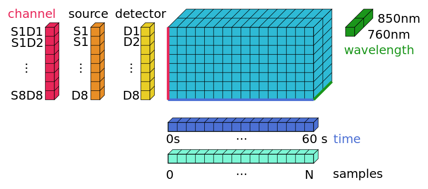
mulitvariate time series are stored in
xarray.DataArraysif it has dimensions ‘channel’ and ‘time’ we call it a
NDTimeSeriesnamed dimensions
coordinates
physical units
[9]:
rec["amp"]
[9]:
<xarray.DataArray (channel: 28, wavelength: 2, time: 23239)> Size: 10MB
[V] 0.09137 0.09099 0.09102 0.09044 0.09094 ... 1.277 1.273 1.273 1.273 1.276
Coordinates:
  * time        (time) float64 186kB 0.0 0.128 0.256 ... 2.974e+03 2.974e+03
    samples     (time) int64 186kB 0 1 2 3 4 5 ... 23234 23235 23236 23237 23238
  * channel     (channel) object 224B 'S1D1' 'S1D2' 'S1D3' ... 'S8D8' 'S8D16'
    source      (channel) object 224B 'S1' 'S1' 'S1' 'S1' ... 'S8' 'S8' 'S8'
    detector    (channel) object 224B 'D1' 'D2' 'D3' 'D9' ... 'D7' 'D8' 'D16'
  * wavelength  (wavelength) float64 16B 760.0 850.0
Attributes:
data_type_group: unprocessed raw[10]:
rec["conc"] = calc_concentratoin(rec)
display(rec["conc"])
<xarray.DataArray 'concentration' (chromo: 2, channel: 28, time: 23239)> Size: 10MB
[µM] 0.1336 0.00383 0.3486 0.1915 0.4156 ... -1.037 -1.004 -1.073 -1.067 -1.076
Coordinates:
  * chromo    (chromo) <U3 24B 'HbO' 'HbR'
  * time      (time) float64 186kB 0.0 0.128 0.256 ... 2.974e+03 2.974e+03
    samples   (time) int64 186kB 0 1 2 3 4 5 ... 23234 23235 23236 23237 23238
  * channel   (channel) object 224B 'S1D1' 'S1D2' 'S1D3' ... 'S8D8' 'S8D16'
    source    (channel) object 224B 'S1' 'S1' 'S1' 'S1' ... 'S7' 'S8' 'S8' 'S8'
detector (channel) object 224B 'D1' 'D2' 'D3' 'D9' ... 'D7' 'D8' 'D16'Probe Geometry - geo3D
labeled points stored in 2D array
if it has a ‘label’ dimension and ‘label’ and ‘type’ coordinates we call it
LabeledPoints
[11]:
rec.geo3d
[11]:
<xarray.DataArray (label: 55, digitized: 3)> Size: 1kB
[m] -0.04161 0.0268 0.1299 -0.06477 0.05814 ... 0.06258 0.08226 0.01751 0.06619
Coordinates:
    type     (label) object 440B PointType.SOURCE ... PointType.LANDMARK
  * label    (label) <U3 660B 'S1' 'S2' 'S3' 'S4' 'S5' ... '25' '26' '27' '28'
Dimensions without coordinates: digitizedXarray functionality
Specify axis by name:
[12]:
amp = rec["amp"]

amp.mean("time")
[12]:
<xarray.DataArray (channel: 28, wavelength: 2)> Size: 448B
[V] 0.09514 0.1902 0.2256 0.6123 0.1177 ... 0.485 0.5704 0.9371 0.6681 1.259
Coordinates:
  * channel     (channel) object 224B 'S1D1' 'S1D2' 'S1D3' ... 'S8D8' 'S8D16'
    source      (channel) object 224B 'S1' 'S1' 'S1' 'S1' ... 'S8' 'S8' 'S8'
    detector    (channel) object 224B 'D1' 'D2' 'D3' 'D9' ... 'D7' 'D8' 'D16'
* wavelength (wavelength) float64 16B 760.0 850.0get the second channel formed by S1 and D2:
[13]:
amp[1, :, :] # location-based indexing
amp.loc["S1D2", :, :] # label-based indexing
amp.sel(channel="S1D2") # label-based indexing
[13]:
<xarray.DataArray (wavelength: 2, time: 23239)> Size: 372kB
[V] 0.2275 0.2297 0.2261 0.2259 0.2267 ... 0.6126 0.6136 0.6072 0.6087 0.6091
Coordinates:
  * time        (time) float64 186kB 0.0 0.128 0.256 ... 2.974e+03 2.974e+03
    samples     (time) int64 186kB 0 1 2 3 4 5 ... 23234 23235 23236 23237 23238
    channel     <U4 16B 'S1D2'
    source      object 8B 'S1'
    detector    object 8B 'D2'
  * wavelength  (wavelength) float64 16B 760.0 850.0
Attributes:
data_type_group: unprocessed rawJoins between two arrays:
[14]:
rec.geo3d.loc[amp.source]
[14]:
<xarray.DataArray (channel: 28, digitized: 3)> Size: 672B
[m] -0.04161 0.0268 0.1299 -0.04161 0.0268 ... 0.06571 0.08189 0.02043 0.06571
Coordinates:
    type      (channel) object 224B PointType.SOURCE ... PointType.SOURCE
    label     (channel) <U3 336B 'S1' 'S1' 'S1' 'S1' ... 'S7' 'S8' 'S8' 'S8'
  * channel   (channel) object 224B 'S1D1' 'S1D2' 'S1D3' ... 'S8D8' 'S8D16'
    source    (channel) object 224B 'S1' 'S1' 'S1' 'S1' ... 'S7' 'S8' 'S8' 'S8'
    detector  (channel) object 224B 'D1' 'D2' 'D3' 'D9' ... 'D7' 'D8' 'D16'
Dimensions without coordinates: digitized[15]:
distances = xrutils.norm(rec.geo3d.loc[amp.source] - rec.geo3d.loc[amp.detector], "digitized")
display(distances)
<xarray.DataArray (channel: 28)> Size: 224B
[m] 0.03929 0.03891 0.04089 0.00826 0.03718 ... 0.00732 0.04067 0.03344 0.007534
Coordinates:
  * channel   (channel) object 224B 'S1D1' 'S1D2' 'S1D3' ... 'S8D8' 'S8D16'
    source    (channel) object 224B 'S1' 'S1' 'S1' 'S1' ... 'S7' 'S8' 'S8' 'S8'
detector (channel) object 224B 'D1' 'D2' 'D3' 'D9' ... 'D7' 'D8' 'D16'Physical units:
[16]:
rec.masks["distance_mask"] = distances > 1.5 * cedalion.units.cm
display(rec.masks["distance_mask"])
<xarray.DataArray (channel: 28)> Size: 28B
True True True False True True True ... False True True False True True False
Coordinates:
  * channel   (channel) object 224B 'S1D1' 'S1D2' 'S1D3' ... 'S8D8' 'S8D16'
    source    (channel) object 224B 'S1' 'S1' 'S1' 'S1' ... 'S7' 'S8' 'S8' 'S8'
detector (channel) object 224B 'D1' 'D2' 'D3' 'D9' ... 'D7' 'D8' 'D16'Additional functionality through accessors:
[17]:
distances.pint.to("mm")
[17]:
<xarray.DataArray (channel: 28)> Size: 224B
[mm] 39.29 38.91 40.89 8.26 37.18 37.6 ... 40.43 37.22 7.32 40.67 33.44 7.534
Coordinates:
  * channel   (channel) object 224B 'S1D1' 'S1D2' 'S1D3' ... 'S8D8' 'S8D16'
    source    (channel) object 224B 'S1' 'S1' 'S1' 'S1' ... 'S7' 'S8' 'S8' 'S8'
detector (channel) object 224B 'D1' 'D2' 'D3' 'D9' ... 'D7' 'D8' 'D16'Writing snirf files
pass
Recordingobject tocedalion.io.write_snirfcaveat: many
Recordingfields have correspondants in snirf files, but not all.
[18]:
with tempfile.TemporaryDirectory() as tmpdir:
    output_path = Path(tmpdir).joinpath("test.snirf")

    cedalion.io.write_snirf(output_path, rec)
Summary
In this notebook you have seen Cedalion’s three primary data types:
Type |
xarray type |
Key dimensions |
Purpose |
|---|---|---|---|
|
|
|
Timeseries data with labels and units |
|
|
|
Optode/landmark 3-D positions |
|
Python dataclass |
— |
Session container: timeseries, geometry, stim, masks |
Key takeaways:
Use
.sel()and.loc[]to index by label rather than by position.Canonical timeseries keys (
"amp","od","conc") are used byread_snirfandwrite_snirf; you can add your own under any name.Physical units are attached via pint-xarray (
.pint.quantify(),.pint.to()); always check that units are preserved after array operations.
Next steps: see the Quick Start guide for a complete preprocessing pipeline, or jump directly into the Tutorial Notebooks.
References
[19]:
cedalion.bib.dump_to_notebook()
Methods used
| [1] | Luke2021 | cedalion.data.get_fingertapping, cedalion.data.get_fingertapping_snirf_path | Robert Luke and David McAlpine. fNIRS Finger Tapping Data in BIDS Format. September 2021. doi:10.5281/zenodo.5529797. |
| [2] | Tucker2022 | cedalion.io.snirf.read_snirf | Stephen Tucker, Jay Dubb, Sreekanth Kura, Alexander von Lühmann, Robert Franke, Jörn M. Horschig, Samuel Powell, Robert Oostenveld, Michael Lührs, Édouard Delaire, Zahra M. Aghajan, Hanseok Yun, Meryem A. Yücel, Qianqian Fang, Theodore J. Huppert, Blaise deB. Frederick, Luca Pollonini, David A. Boas, and Robert Luke. Introduction to the shared near infrared spectroscopy format. Neurophotonics, 10(1):013507, 2022. doi:10.1117/1.NPh.10.1.013507. |
| [3] | Delpy1988 | cedalion.nirs.cw.int2od, cedalion.nirs.cw.od2conc | D. T. Delpy, M. Cope, P. van der Zee, S. Arridge, S. Wray, and J. Wyatt. Estimation of optical pathlength through tissue from direct time of flight measurement. Physics in Medicine and Biology, 33(12):1433–1442, 1988. doi:10.1088/0031-9155/33/12/008. |
| [4] | Villringer1997 | cedalion.nirs.cw.int2od, cedalion.nirs.cw.od2conc | Arno Villringer and Britton Chance. Non-invasive optical spectroscopy and imaging of human brain function. Trends in Neurosciences, 20(10):435–442, 1997. doi:10.1016/S0166-2236(97)01132-6. |
| [5] | Prahl1998 | cedalion.nirs.common.get_extinction_coefficients | Scott A. Prahl. Optical absorption of hemoglobin. Oregon Medical Laser Center, online resource, 1998. URL: https://omlc.org/spectra/hemoglobin/. |