S4: Model-driven (GLM) Analysis
This tutorial demonstrates how to use a General Linear Model (GLM) to model the recorded time series as a superposition of hemodynamic responses and nuisance effects.
Learning objectives
In this notebook you will learn to:
Build a GLM design matrix with HRF, drift, and short-channel regressors
Fit the GLM per channel using AR-IRLS and inspect beta coefficients
Visualise channel-space activation maps on a scalp topography
Understand the role of short-separation channel regression for noise removal
[1]:
# This cells setups the environment when executed in Google Colab.
try:
    import google.colab
    !curl -s https://raw.githubusercontent.com/ibs-lab/cedalion/dev/scripts/colab_setup.py -o colab_setup.py
    # Select branch with --branch "branch name" (default is "dev")
    %run colab_setup.py
except ImportError:
    pass
[2]:
import cedalion
import cedalion.sigproc.quality as quality
import cedalion.sigproc.motion as motion
import cedalion.sigproc.physio as physio


from cedalion import units
import cedalion.xrutils as xrutils
import cedalion.models.glm as glm
import cedalion.data

import cedalion.vis.blocks as vbx
from cedalion.vis.anatomy import scalp_plot, plot_montage3D
from cedalion.vis.colors import p_values_cmap

import numpy as np
import xarray as xr

import matplotlib.pyplot as p
from statsmodels.stats.multitest import multipletests

xr.set_options(display_expand_data=False)
xrutils.unit_stripping_is_error()
Load Data
The dataset is loaded and events are renamed. Afterwards, the stimulus data frame is summarized.
[3]:
rec = cedalion.data.get_fingertappingDOT()

# assign better trial_type labels
rec.stim.cd.rename_events(
    {
        "1": "Control",
        "2": "FTapping/Left",
        "3": "FTapping/Right",
        "4": "BallSqueezing/Left",
        "5": "BallSqueezing/Right",
    }
)
[4]:
# count trials
rec.stim.groupby("trial_type")[["trial_type"]].count().rename(
    {"trial_type": "# trials"},
    axis=1,
)
[4]:
| # trials | |
|---|---|
| trial_type | |
| BallSqueezing/Left | 17 |
| BallSqueezing/Right | 16 |
| Control | 65 |
| FTapping/Left | 16 |
| FTapping/Right | 16 |
Trim dataset
Trim the dataset to roughly 5 minutes to keep computation times low while still preserving three trials per condition. Also exclude the ‘BallSqueezing’ conditions.
[5]:
tmin = 5
tmax = 315

rec.stim = rec.stim[
    (tmin <= rec.stim.onset)
    & (rec.stim.onset <= tmax)
    & (rec.stim.trial_type.isin(["Control", "FTapping/Left", "FTapping/Right"]))
]
# use a slice to select a time range
rec["amp_cropped"] = rec["amp"].sel(time=slice(tmin,tmax))

# count remaining trials
rec.stim.groupby("trial_type")[["trial_type"]].count().rename(
    {"trial_type": "# trials"},
    axis=1,
)
[5]:
| # trials | |
|---|---|
| trial_type | |
| Control | 10 |
| FTapping/Left | 3 |
| FTapping/Right | 3 |
Preprocessing
The same motion-correction methods as described in the third tutorial notebook are applied, and the bad channels identified there are removed. The cleaned optical-density time series are then converted to concentration changes. Finally, a low-pass filter with a 0.5 Hz cutoff is applied to remove the cardiac component.
[6]:
rec["od"] = cedalion.nirs.cw.int2od(rec["amp_cropped"])
rec["od_tddr"] = motion.tddr(rec["od"])
rec["od_wavelet"] = motion.wavelet(rec["od_tddr"])

bad_channels = ['S13D26', 'S14D28']

rec["od_clean"] = rec["od_wavelet"].sel(channel=~rec["od"].channel.isin(bad_channels))

# differential pathlength factors
dpf = xr.DataArray(
    [6, 6],
    dims="wavelength",
    coords={"wavelength": rec["amp"].wavelength},
)

rec["conc"] = cedalion.nirs.cw.od2conc(rec["od_clean"], rec.geo3d, dpf, spectrum="prahl")

# Here we use a lowpass-filter to remove the cardiac component.
# Drift will be modeled in the design matrix.

fmin = 0 * units.Hz
fmax = 0.5 * units.Hz

rec["conc_filtered"] = cedalion.sigproc.frequency.freq_filter(rec["conc"], fmin, fmax)

TS_NAME = "conc_filtered"
[7]:
display(rec[TS_NAME])
<xarray.DataArray 'concentration' (chromo: 2, channel: 98, time: 1352)> Size: 2MB
[µM] 0.8276 0.7548 0.7043 0.6868 0.6978 ... -0.08036 -0.07753 -0.07426 -0.07086
Coordinates:
  * chromo    (chromo) <U3 24B 'HbO' 'HbR'
  * time      (time) float64 11kB 5.046 5.276 5.505 5.734 ... 314.5 314.7 314.9
    samples   (time) int64 11kB 22 23 24 25 26 27 ... 1369 1370 1371 1372 1373
  * channel   (channel) object 784B 'S1D1' 'S1D2' 'S1D4' ... 'S14D31' 'S14D32'
    source    (channel) object 784B 'S1' 'S1' 'S1' 'S1' ... 'S14' 'S14' 'S14'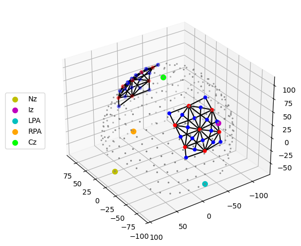
detector (channel) object 784B 'D1' 'D2' 'D4' 'D5' ... 'D29' 'D31' 'D32'Montage and Channel Distances
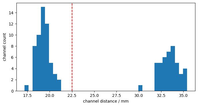
The hexagonal montage has longer (3-3.5cm) and shorter (~1.7-2.2cm) channels. We define a cut-off at 22.5 mm to separate long and short channels.
[8]:
plot_montage3D(rec["amp"], rec.geo3d)
Calculate and histogram channel distances:
[9]:
distances = cedalion.nirs.channel_distances(rec["amp"], rec.geo3d)

p.figure(figsize=(8,4))
p.hist(distances, 40)
p.axvline(22.5, c="r", ls="--")
p.xlabel("channel distance / mm")
p.ylabel("channel count");
Split long and short channels
[10]:
rec["ts_long"], rec["ts_short"] = cedalion.nirs.split_long_short_channels(
    rec[TS_NAME], rec.geo3d, distance_threshold=22.5 * units.mm
)

# This renaming is for display purposes only.
display(rec["ts_long"].rename("long channels"))
display(rec["ts_short"].rename("short channels"))
<xarray.DataArray 'long channels' (chromo: 2, channel: 44, time: 1352)> Size: 952kB
[µM] 0.3715 0.3284 0.2975 0.2849 0.2892 ... 0.006362 0.008495 0.01122 0.01438
Coordinates:
  * chromo    (chromo) <U3 24B 'HbO' 'HbR'
  * time      (time) float64 11kB 5.046 5.276 5.505 5.734 ... 314.5 314.7 314.9
    samples   (time) int64 11kB 22 23 24 25 26 27 ... 1369 1370 1371 1372 1373
  * channel   (channel) object 352B 'S1D6' 'S1D8' 'S2D5' ... 'S14D25' 'S14D27'
    source    (channel) object 352B 'S1' 'S1' 'S2' 'S2' ... 'S13' 'S14' 'S14'
detector (channel) object 352B 'D6' 'D8' 'D5' 'D9' ... 'D28' 'D25' 'D27'<xarray.DataArray 'short channels' (chromo: 2, channel: 54, time: 1352)> Size: 1MB
[µM] 0.8276 0.7548 0.7043 0.6868 0.6978 ... -0.08036 -0.07753 -0.07426 -0.07086
Coordinates:
* chromo (chromo) <U3 24B 'HbO' 'HbR'
* time (time) float64 11kB 5.046 5.276 5.505 5.734 ... 314.5 314.7 314.9
samples (time) int64 11kB 22 23 24 25 26 27 ... 1369 1370 1371 1372 1373
* channel (channel) object 432B 'S1D1' 'S1D2' 'S1D4' ... 'S14D31' 'S14D32'
source (channel) object 432B 'S1' 'S1' 'S1' 'S1' ... 'S14' 'S14' 'S14'
detector (channel) object 432B 'D1' 'D2' 'D4' 'D5' ... 'D29' 'D31' 'D32'Fitting a General Linear Model
The GLM for fNIRS explains the time series (Y) for each channel and chromophore individually as a linear superposition of regressors, some representing the hemodynamic response and others addressing nuisance effects such as superficial or physiological components and signal drifts. The regressors form the design matrix (G) and the fit determines the unknown coefficients (β) for each regressor in the presence of unmodeled noise (E).
Building the Design Matrix
The design matrix comprises the hemodynamic response, short channel and drift regressors.
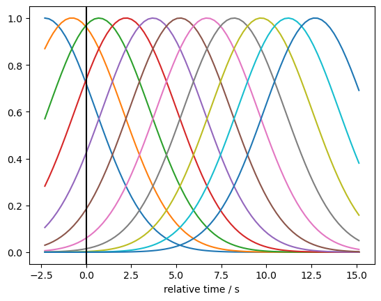
We model the hemodynamic response function (HRF) using a set of Gaussian basis kernels. The basis is defined by the durations of pre- and post-stimulus periods, the temporal spacing between successive kernels, and the standard deviation (width) of each Gaussian.
Using an instance of cedalion.models.glm.basis_functions.GaussianKernels, a basis for the long-channel time series is created and visualized.
[11]:
gaussian_kernels = glm.basis_functions.GaussianKernels(
    t_pre=2 * units.s,
    t_post=15 * units.s,
    t_delta=1.5 * units.s,
    t_std=2 * units.s,
)

hrf_basis = gaussian_kernels(rec["ts_long"])

for i in range(hrf_basis.sizes["component"]):
    p.plot(hrf_basis.time, hrf_basis[:,i])
    p.xlabel("relative time / s")
p.axvline(0, c="k")
[11]:
<matplotlib.lines.Line2D at 0x7f202e696ad0>
In Cedalion the class glm.DesignMatrix manages the regressors.
Functions in the package glm.design_matrix create regressors and return them as instances of DesignMatrix. These can be combined with the &-operator.
In this example, all short channels are averaged to model a global (mostly) superficial component.
Any remaining signal drift is modeled with cosine basis functions up tp 0.02 Hz.
[12]:
dms = (
    glm.design_matrix.hrf_regressors(
        rec["ts_long"],
        rec.stim,
        gaussian_kernels,
    )
    & glm.design_matrix.drift_cosine_regressors(rec[TS_NAME], fmax=0.02 * units.Hz)
    & glm.design_matrix.average_short_channel_regressor(rec["ts_short"])
)
When fitting a GLM to fNIRS data, some regressors are shared across all channels, wheras others are channel-specific. For example, if superficial physiology is modeled using the nearest short-separation channel for each measurement channel, the resulting short-channel regressor is channel-specific and therefore differs across channels.
Consequently, the DesignMatrix distinguishes between common regressors and channel-wise regressors. In this example the design matrix has only common regressors.
Each regressor has a string label for clarity. The convention used by Cedalion is to use labels of the form 'HRF <trial_typ> <number>' for the HRF regressors and 'Drift <type> <number>' for the drift components.
As with the trial-type labels, adopting this naming scheme makes it straightforward to select regressors. In this instance, the stimulus ‘BallSqueezing/Left’ is modeled with multiple regressors. They can be easily distinguished from other HRF or drift terms by selecting labels that begin with ‘HRF BallSqueezing/Left’.
[13]:
display(dms)
display(dms.common)
display(dms.channel_wise)
DesignMatrix(common=['HRF Control 00','HRF Control 01','HRF Control 02','HRF Control 03','HRF Control 04','HRF Control 05','HRF Control 06','HRF Control 07','HRF Control 08','HRF Control 09','HRF Control 10','HRF FTapping/Left 00','HRF FTapping/Left 01','HRF FTapping/Left 02','HRF FTapping/Left 03','HRF FTapping/Left 04','HRF FTapping/Left 05','HRF FTapping/Left 06','HRF FTapping/Left 07','HRF FTapping/Left 08','HRF FTapping/Left 09','HRF FTapping/Left 10','HRF FTapping/Right 00','HRF FTapping/Right 01','HRF FTapping/Right 02','HRF FTapping/Right 03','HRF FTapping/Right 04','HRF FTapping/Right 05','HRF FTapping/Right 06','HRF FTapping/Right 07','HRF FTapping/Right 08','HRF FTapping/Right 09','HRF FTapping/Right 10','Drift Cos 0','Drift Cos 1','Drift Cos 2','Drift Cos 3','Drift Cos 4','Drift Cos 5','Drift Cos 6','Drift Cos 7','Drift Cos 8','Drift Cos 9','Drift Cos 10','Drift Cos 11','short'], channel_wise=[])
<xarray.DataArray (time: 1352, regressor: 46, chromo: 2)> Size: 995kB
0.0 0.0 0.0 0.0 0.0 0.0 0.0 ... 0.9999 0.9999 -0.9999 -0.9999 0.4137 0.03177
Coordinates:
  * time       (time) float64 11kB 5.046 5.276 5.505 5.734 ... 314.5 314.7 314.9
  * regressor  (regressor) <U21 4kB 'HRF Control 00' ... 'short'
  * chromo     (chromo) <U3 24B 'HbO' 'HbR'
    samples    (time) int64 11kB 22 23 24 25 26 27 ... 1369 1370 1371 1372 1373
[]
Visualize the design matrix
[14]:
# select common regressors
dm = dms.common
display(dm)

# using xr.DataArray.plot
f, ax = p.subplots(1,1,figsize=(12,10))
dm.sel(chromo="HbO", time=dm.time < 600).T.plot()
p.title("Shared Regressors")
p.show()
<xarray.DataArray (time: 1352, regressor: 46, chromo: 2)> Size: 995kB
0.0 0.0 0.0 0.0 0.0 0.0 0.0 ... 0.9999 0.9999 -0.9999 -0.9999 0.4137 0.03177
Coordinates:
  * time       (time) float64 11kB 5.046 5.276 5.505 5.734 ... 314.5 314.7 314.9
  * regressor  (regressor) <U21 4kB 'HRF Control 00' ... 'short'
  * chromo     (chromo) <U3 24B 'HbO' 'HbR'
    samples    (time) int64 11kB 22 23 24 25 26 27 ... 1369 1370 1371 1372 1373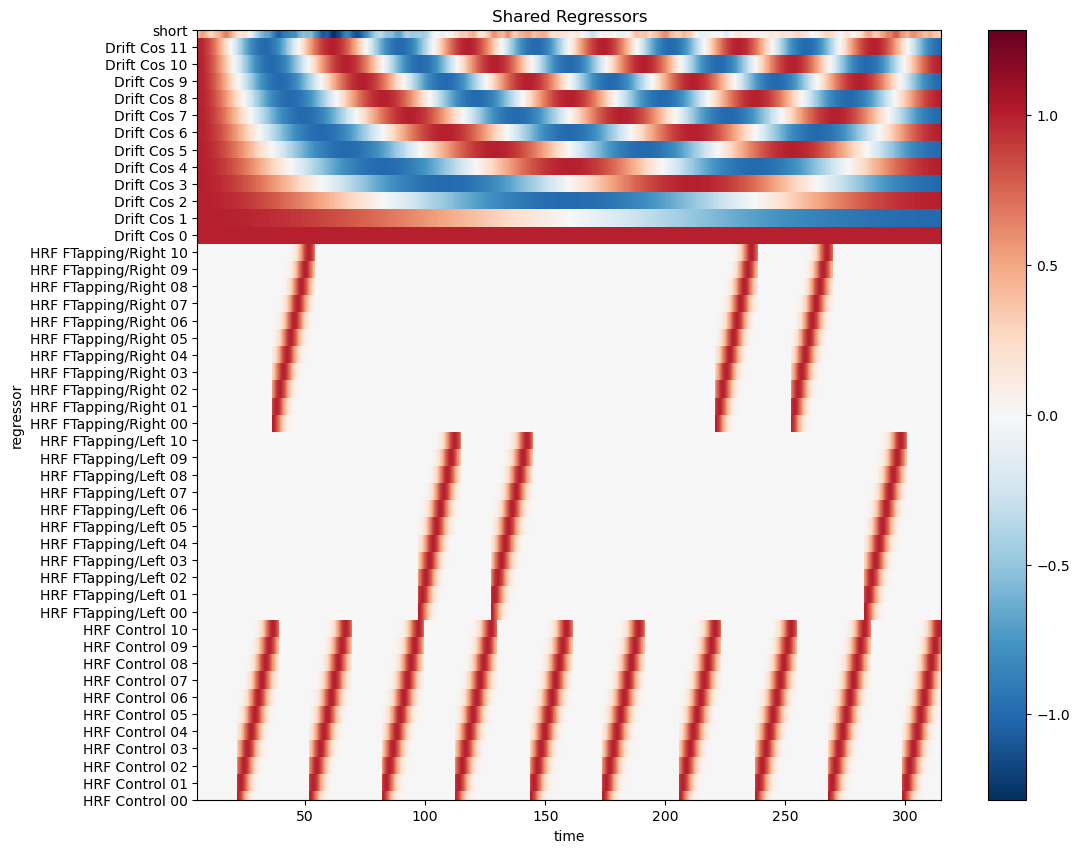
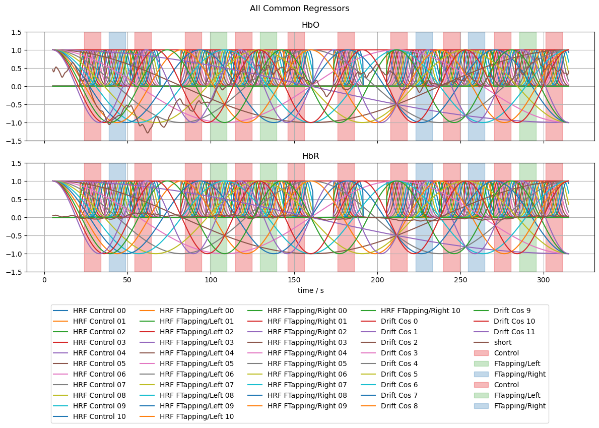
[15]:
# line plots of all regressors
f, ax = p.subplots(2,1,sharex=True, figsize=(12,6))

for i, chromo in enumerate(["HbO", "HbR"]):
    for reg in dm.regressor.values:
        label = reg if i == 0 else None
        ax[i].plot(dm.time, dm.sel(chromo=chromo, regressor=reg), label=label)

    vbx.plot_stim_markers(ax[i], rec.stim, y=1)
    ax[i].grid()
    ax[i].set_title(chromo)
    ax[i].set_ylim(-1.5,1.5)
f.suptitle("All Common Regressors")

f.legend(ncol=5, loc="upper center", bbox_to_anchor=(0.5, 0))
#ax[0].set_xlim(0,240);
ax[1].set_xlabel("time / s");
f.set_tight_layout(True)
Fitting the Model
To fit the GLM, use glm.fit, which requires the time series and the design matrix as inputs. Optionally, you can choose a noise model from the following currently supported options:
ols (default): ordinary least squares
rls: recursive least squares
wls: weighted least squares
ar_irls: autoregressive iteratively reweighted least squares
gls: generalized least squares
glsar: generalized least squares with autoregressive covariance structure
Model fitting is implemented using the statsmodels library. Because each channel-chromophore pair is fitted independently, the output consists of one statsmodels.RegressionResults object per channel and chromophore. These are arranged in a DataArray object with dimensions ('channel', 'chromo').
The user can investigate fit results, assess parameter uncertainties and perform hypothesis tests through functions of the RegressionResults objects. To facilitate calling these functions on all result objects in a DataArray, Cedalion provides the .sm accessor. For example, model coefficients (betas) can be obtained with result.sm.params, which calls params on all result objects and returns a DataArray with the parameters. For the full list of available methods and
attributes, see the statsmodels documentation. .
[16]:
#results = glm.fit(rec["ts_long"], dms, noise_model="ols", max_jobs=-1)
results = glm.fit(rec["ts_long"], dms, noise_model="ar_irls", max_jobs=-1)

display(results)
 98%|█████████▊| 43/44 [02:00<00:02,  2.80s/it]
 98%|█████████▊| 43/44 [01:30<00:02,  2.11s/it]
<xarray.DataArray (channel: 44, chromo: 2)> Size: 704B
<statsmodels.robust.robust_linear_model.RLMResultsWrapper object at 0x7f202d1...
Coordinates:
  * chromo    (chromo) <U3 24B 'HbO' 'HbR'
  * channel   (channel) object 352B 'S1D6' 'S1D8' 'S2D5' ... 'S14D25' 'S14D27'
    source    (channel) object 352B 'S1' 'S1' 'S2' 'S2' ... 'S13' 'S14' 'S14'
    detector  (channel) object 352B 'D6' 'D8' 'D5' 'D9' ... 'D28' 'D25' 'D27'
Attributes:
description: AR_IRLSInspecting Fit Results
The result of the fit is an array of statsmodels result objects. Each contains the fitted parameters and other functionality to inspect fit parameter uncertainty or to perform hypothesis tests.
[17]:
results[0,0].item().params
[17]:
HRF Control 00            0.276679
HRF Control 01           -1.322791
HRF Control 02            3.381821
HRF Control 03           -5.959108
HRF Control 04            7.910174
HRF Control 05           -8.189405
HRF Control 06            6.586288
HRF Control 07           -4.007499
HRF Control 08            1.722847
HRF Control 09           -0.484760
HRF Control 10            0.070155
HRF FTapping/Left 00      0.234327
HRF FTapping/Left 01     -0.918640
HRF FTapping/Left 02      1.663889
HRF FTapping/Left 03     -1.340174
HRF FTapping/Left 04     -0.837867
HRF FTapping/Left 05      3.703105
HRF FTapping/Left 06     -4.886997
HRF FTapping/Left 07      3.755480
HRF FTapping/Left 08     -1.792997
HRF FTapping/Left 09      0.528106
HRF FTapping/Left 10     -0.077728
HRF FTapping/Right 00    -0.858642
HRF FTapping/Right 01     4.243696
HRF FTapping/Right 02   -11.265726
HRF FTapping/Right 03    20.680841
HRF FTapping/Right 04   -28.569770
HRF FTapping/Right 05    30.562608
HRF FTapping/Right 06   -25.349188
HRF FTapping/Right 07    15.793779
HRF FTapping/Right 08    -6.882461
HRF FTapping/Right 09     1.949848
HRF FTapping/Right 10    -0.283047
Drift Cos 0               0.019738
Drift Cos 1              -0.062680
Drift Cos 2              -0.048399
Drift Cos 3              -0.004764
Drift Cos 4               0.098752
Drift Cos 5               0.038450
Drift Cos 6               0.049932
Drift Cos 7               0.015421
Drift Cos 8               0.003108
Drift Cos 9               0.050348
Drift Cos 10              0.032108
Drift Cos 11             -0.038858
short                     0.654660
dtype: float64
Cedalion provides the .sm accessor on arrays of result objects to make accessing the statsmodels functionality easier.
[18]:
display(results.sm.params)
<xarray.DataArray (channel: 44, chromo: 2, regressor: 46)> Size: 32kB
0.2767 -1.323 3.382 -5.959 7.91 ... -0.008269 -0.0007833 0.01253 0.01076 0.2799
Coordinates:
  * regressor  (regressor) object 368B 'HRF Control 00' ... 'short'
  * chromo     (chromo) <U3 24B 'HbO' 'HbR'
  * channel    (channel) object 352B 'S1D6' 'S1D8' 'S2D5' ... 'S14D25' 'S14D27'
    source     (channel) object 352B 'S1' 'S1' 'S2' 'S2' ... 'S13' 'S14' 'S14'
    detector   (channel) object 352B 'D6' 'D8' 'D5' 'D9' ... 'D28' 'D25' 'D27'
Attributes:
description: AR_IRLSThe glm.predict function takes the original time series, the design matrix and the fitted parameters. Using these it predicts the sum of all regressors scaled with the best fitted parameters.
When only a subset of the fitted parameters is provided, only those regressors are considered. This allows to predict the signal or background components separately.
[19]:
predicted = glm.predict(rec["ts_long"], results.sm.params, dms)

predicted_background = glm.predict(
    rec["ts_long"],
    results.sm.params.sel(
        regressor=results.sm.params.regressor.str.startswith("Drift")
        | results.sm.params.regressor.str.startswith("short")
    ),
    dms,
)
predicted_signal = glm.predict(
    rec["ts_long"],
    results.sm.params.sel(regressor=results.sm.params.regressor.str.startswith("HRF")),
    dms,
)

meas_hrf_only = rec["ts_long"].pint.dequantify() - predicted_background
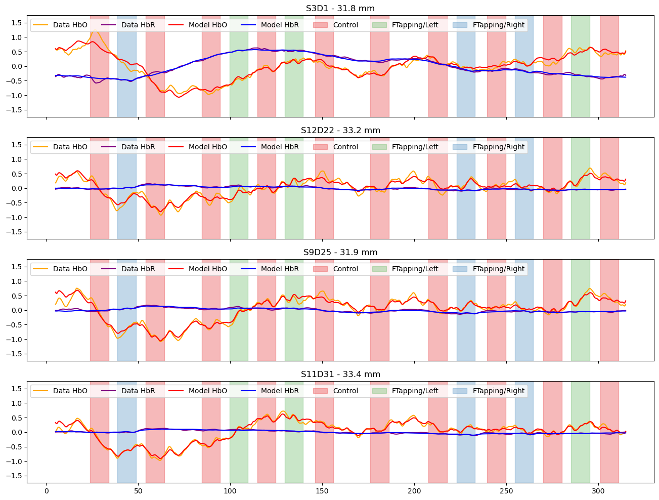
Compare the preprocessed data to the full model
[20]:
channels = ["S3D1", "S12D22", "S9D25", "S11D31"]

f, ax = p.subplots(len(channels),1, figsize=(16, 3*len(channels)), sharex=True)

for i_ch, ch in enumerate(channels):
    ax[i_ch].plot(rec["ts_long"].time, rec["ts_long"].sel(channel=ch, chromo="HbO"), "-", c="orange", label="Data HbO")
    ax[i_ch].plot(rec["ts_long"].time, rec["ts_long"].sel(channel=ch, chromo="HbR"), "-", c="purple", label="Data HbR")
    ax[i_ch].plot(predicted_background.time, predicted.sel(channel=ch, chromo="HbO"), "r-", label="Model HbO")
    ax[i_ch].plot(predicted_background.time, predicted.sel(channel=ch, chromo="HbR"), "b-", label="Model HbR")
    vbx.plot_stim_markers(ax[i_ch], rec.stim, y=1)
    ax[i_ch].set_title(f"{ch} - {distances.sel(channel=ch).item().magnitude:.1f} mm")
    ax[i_ch].set_ylim(-1.75,1.75)
    ax[i_ch].legend(loc="upper left", ncol=8)
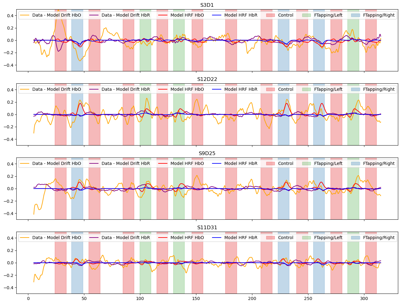
Subtract the components modelled by short and drift regressors and show the fitted activations
[21]:
f, ax = p.subplots(len(channels),1, figsize=(16, 3*len(channels)), sharex=True)

for i_ch, ch in enumerate(channels):
    ax[i_ch].plot(meas_hrf_only.time, meas_hrf_only.sel(channel=ch, chromo="HbO"), "-", c="orange", label="Data - Model Drift HbO" )
    ax[i_ch].plot(meas_hrf_only.time, meas_hrf_only.sel(channel=ch, chromo="HbR"), "-", c="purple", label="Data - Model Drift HbR")
    ax[i_ch].plot(predicted_signal.time, predicted_signal.sel(channel=ch, chromo="HbO"), "r-", label="Model HRF HbO")
    ax[i_ch].plot(predicted_signal.time, predicted_signal.sel(channel=ch, chromo="HbR"), "b-", label="Model HRF HbR")
    vbx.plot_stim_markers(ax[i_ch], rec.stim, y=1)

    ax[i_ch].legend(loc="upper left", ncol=8)
    ax[i_ch].set_title(ch)
    #ax[i_ch].set_ylim(-1.25, 1.25)
    ax[i_ch].set_ylim(-.5, .5)
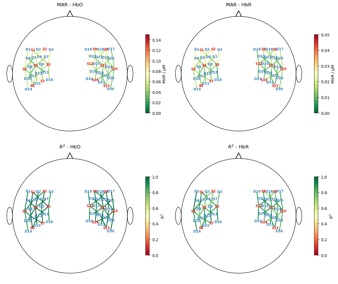
Plot goodness of fit metrics
To assess how well the fitted model describes the data, to metrics are calculated and visualized in scalp plots
the median absolute residuals (MAR) and
the coefficient of determination \(R^2\)
Note the scale difference between HbO and HbR for the MAR metric.
[22]:
mar = np.abs(predicted - rec["ts_long"].pint.dequantify()).median("time")

ss_res = ((rec["ts_long"].pint.dequantify() - predicted)**2).sum("time")
ss_tot = ((rec["ts_long"] - rec["ts_long"].mean("time"))**2).pint.dequantify().sum("time")
r2 = (1 - ss_res / ss_tot)

f,ax = p.subplots(2,2, figsize=(12,10))

for i, chromo in enumerate(["HbO", "HbR"]):
    scalp_plot(
        rec["ts_long"],
        rec.geo3d,
        # results.sm.pvalues.sel(regressor=reg, chromo=chromo),
        mar.sel(chromo=chromo),
        ax[0,i],
        cmap="RdYlGn_r",
        vmin=0,
        vmax={"HbO" : 0.15, "HbR" : 0.05}[chromo],
        title=f"MAR - {chromo}",
        cb_label="MAR / µM",
        channel_lw=2,
        optode_labels=True,
        optode_size=24,
    )
    scalp_plot(
        rec["ts_long"],
        rec.geo3d,
        r2.sel(chromo=chromo),
        ax[1,i],
        cmap="RdYlGn",
        vmin=0,
        vmax=1,
        title=f"$R^2$ - {chromo}",
        cb_label="$R^2$",
        channel_lw=2,
        optode_labels=True,
        optode_size=24,
    )

f.set_tight_layout(True)
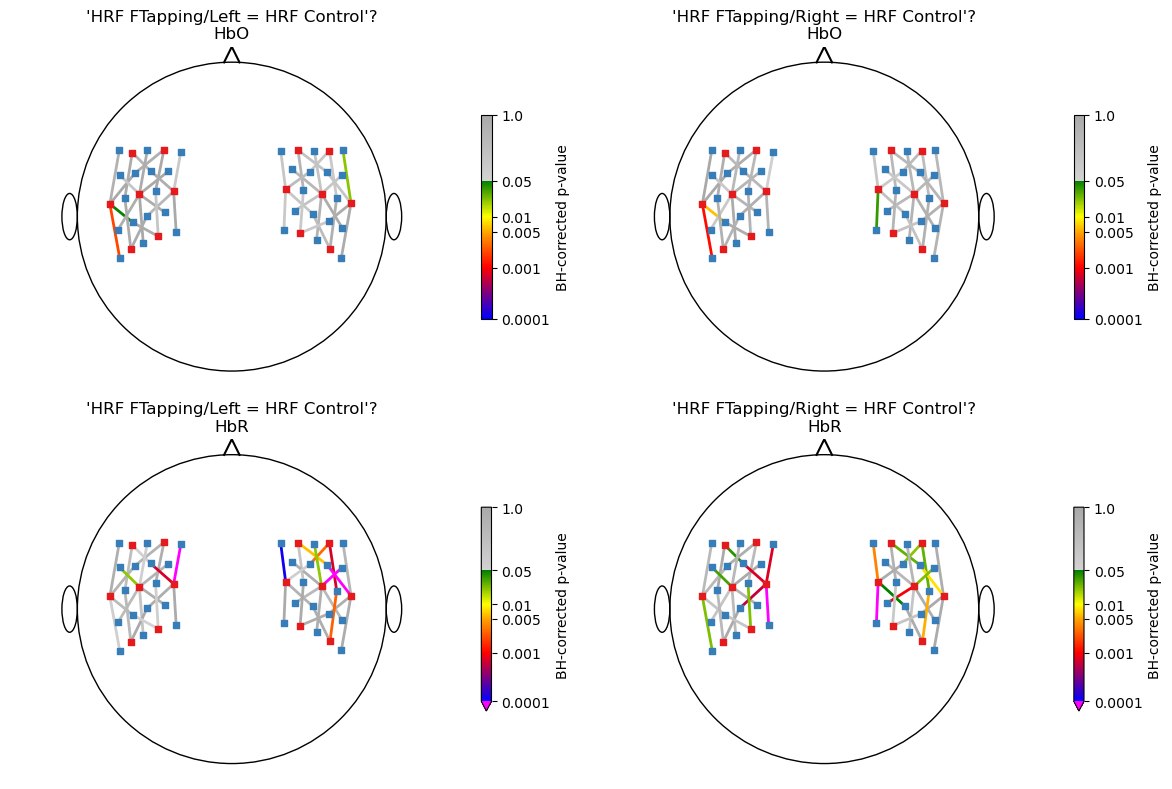
Hypothesis tests
We would like to investigate which channels show activation during finger tapping. Answering this question with a hypothesis test requires specifying a null hypothesis. In this case, the null hypothesis states that the size of the activation during left- or right-hand finger tapping does not differ from the control condition.
For simple models with one regressor per condition, statsmodels provides a convenient interface for formulating such null hypotheses directly.
But in the present case, the HRF for each condition is modeled using multiple Gaussian kernels and the size of the activation needs to be formalized.
The null hypothesis H0 can be formulated as a linear combination of the fitted parameters \(\beta_i\) and a contrast vector \(c_i\) which should be zero if the null hypothesis is true. For example, in a fit with only three parameters, this would look like:
Through the specification of different contrast vectors, different hypothesis can be formulated. For example:
i.e the contrast vector encodes the hypothesis that there is no difference between \(\beta_1\) and \(\beta_3\).
Each such hypothesis is then tested, by checking if the linear combination significantly deviates from zero.
In the present case, we define the size of the activation as the area under the HRF. Because the model is linear, the area under the fitted HRF can be computed as a weighted sum of the Gaussian kernel areas \(A_i\), with the weights given by the fitted parameters \(\beta_i\):
Comparing with the formulas above, it becomes clear that by using the areas of the kernel basis functions as contrast weights and by assigning opposite signs to the conditions being compared, we can formulate the null hypothesis that the size of the activation (as quantified by HRF area) does not differ between two conditions.
Finally, we restrict the area computation to a time window in which the main hemodynamic response is expected, so that the calculated area reflects the activation of interest rather than unrelated fluctuations.
The following cell defines a function that computes contrast vectors from the HRF areas during 5 to 10 seconds post-stimulus then uses this function to formulate the two hypotheses:
“HRF FTapping/Left = HRF Control” and
“HRF FTapping/Right = HRF Control”.
[23]:
def gaussian_kernel_timewindowed_auc_contrast(
    dms, df_stim, condition1: str, condition2: str, tmin: float, tmax: float
):
    """This function computes contrast vectors based on the time-windowed are of the regressors."""

    time = dms.common.time

    # create two masks, that for each condition contains 1.0 only for
    # time samples between onset+tmin and onset+tmax. All other entries
    # zero
    mask_cond1 = np.zeros(len(time))
    mask_cond2 = np.zeros(len(time))

    for _, row in df_stim.iterrows():
        t1, t2 = row["onset"]+tmin, row["onset"]+tmax
        if row["trial_type"].startswith(condition1):
            mask_cond1[(t1 <= time) & (time <= t2)] = 1.
        if row["trial_type"].startswith(condition2):
            mask_cond2[(t1 <= time) & (time <= t2)] = 1.

    # each gaussian regressor is multiplied with the mask for its condition. This sets
    # all parts of the regressor outside the time window to zero. Through integration the remaining
    # area under the curve is calculated.

    nregressors = dms.common.sizes["regressor"]
    contrast = np.zeros(nregressors)
    for i in range(nregressors):
        if dms.common.regressor.values[i].startswith(f"HRF {condition1}"):
            contrast[i] = np.trapezoid(dms.common[:,i,0]*mask_cond1, dms.common.time)
        if dms.common.regressor.values[i].startswith(f"HRF {condition2}"):
            contrast[i] = - np.trapezoid(dms.common[:,i,0]*mask_cond2, dms.common.time)

    return contrast

hypothesis_labels = [
    "HRF FTapping/Left = HRF Control",
    "HRF FTapping/Right = HRF Control",
]

hypotheses = [
    gaussian_kernel_timewindowed_auc_contrast(dms, rec.stim, "FTapping/Left", "Control", 5, 10),
    gaussian_kernel_timewindowed_auc_contrast(dms, rec.stim, "FTapping/Right", "Control", 5, 10),
]

display(hypotheses)
[array([ -0.38536386,  -1.54846768,  -4.83084777, -11.81761093,
        -22.81664425, -35.12676303, -43.40391258, -43.25178978,
        -34.75902577, -22.41329998, -11.52180284,   0.11269669,
          0.45496975,   1.42568445,   3.50208166,   6.7877193 ,
         10.48759214,  13.0030286 ,  12.99994119,  10.48098719,
          6.78010497,   3.49667564,   0.        ,   0.        ,
          0.        ,   0.        ,   0.        ,   0.        ,
          0.        ,   0.        ,   0.        ,   0.        ,
          0.        ,   0.        ,   0.        ,   0.        ,
          0.        ,   0.        ,   0.        ,   0.        ,
          0.        ,   0.        ,   0.        ,   0.        ,
          0.        ,   0.        ]),
 array([ -0.38536386,  -1.54846768,  -4.83084777, -11.81761093,
        -22.81664425, -35.12676303, -43.40391258, -43.25178978,
        -34.75902577, -22.41329998, -11.52180284,   0.        ,
          0.        ,   0.        ,   0.        ,   0.        ,
          0.        ,   0.        ,   0.        ,   0.        ,
          0.        ,   0.        ,   0.12240493,   0.48687159,
          1.50425073,   3.64608706,   6.97863256,  10.65571472,
         13.06351251,  12.91859368,  10.303389  ,   6.59305506,
          3.36289301,   0.        ,   0.        ,   0.        ,
          0.        ,   0.        ,   0.        ,   0.        ,
          0.        ,   0.        ,   0.        ,   0.        ,
          0.        ,   0.        ])]
Using the calculated contrasts (i.e. hypotheses) t-tests are perforemd in each channel and chromophore. The accessor .sm is used to call the t_test function on all results, yielding a DataArray of ContrastResults:
[24]:
contrast_results = results.sm.t_test(hypotheses)
display(contrast_results)
<xarray.DataArray (channel: 44, chromo: 2)> Size: 704B
                             Test for Constraints                            ...
Coordinates:
  * chromo    (chromo) <U3 24B 'HbO' 'HbR'
  * channel   (channel) object 352B 'S1D6' 'S1D8' 'S2D5' ... 'S14D25' 'S14D27'
    source    (channel) object 352B 'S1' 'S1' 'S2' 'S2' ... 'S13' 'S14' 'S14'
    detector  (channel) object 352B 'D6' 'D8' 'D5' 'D9' ... 'D28' 'D25' 'D27'
Attributes:
description: AR_IRLSInspecting a single contrast result: the two rows labeled ‘c0’ and ‘c1’ correspond to the two hypotheses/contrasts “HRF FTapping/Left = HRF Control” and “HRF FTapping/Right = HRF Control”.
[25]:
display(contrast_results[0,0].item())
<class 'statsmodels.stats.contrast.ContrastResults'>
                             Test for Constraints
==============================================================================
                 coef    std err          z      P>|z|      [0.025      0.975]
------------------------------------------------------------------------------
c0             1.0722      0.886      1.211      0.226      -0.664       2.808
c1             1.4259      0.885      1.611      0.107      -0.309       3.161
==============================================================================
Apply FDR-control and visualize corrected p-values for all channels
In the following, the p-values of all tests are visualized in a scalp plot. A Benjamini-Hochberg FDR correction is applied.
[26]:
# create a colormap for p-values
norm, cmap = p_values_cmap()

nhypo = len(hypotheses)
f, ax = p.subplots(2,len(hypotheses),figsize=(6 * nhypo,8))

for i_row, chromo in enumerate(["HbO", "HbR"]):
    for i_hypo, hypo in enumerate(hypotheses):

        # get p_values for all channels and apply fdr correction
        # use Benjamini-Hochberg here
        p_values = contrast_results.sm.p_values().sel(chromo=chromo, hypothesis=i_hypo)
        _, q_values, _, _ = multipletests(p_values, alpha=0.05, method="fdr_bh")

        scalp_plot(
            rec["ts_long"],
            rec.geo3d,
            np.log10(q_values),
            ax[i_row][i_hypo],
            cmap=cmap,
            norm=norm,
            title=f"'{hypothesis_labels[i_hypo]}'?\n{chromo}",
            cb_label="BH-corrected p-value",
            channel_lw=2,
            optode_labels=False,
            cb_ticks_labels=[(np.log10(i), str(i)) for i in [0.0001, 0.001, 0.005, 0.01, 0.05, 1.]],
            optode_size=24,
        )


f.tight_layout()
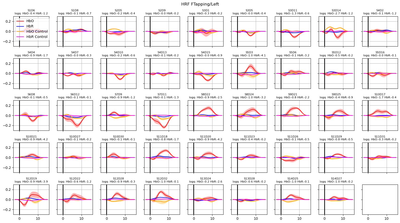
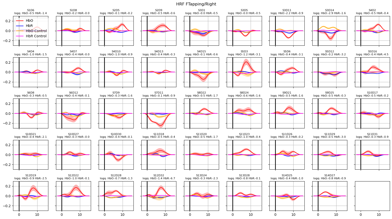
Extract and plot HRFs with uncertainties
For extracting the HRF a special design matrix must be built. It spans only the duration of a single trial, contains only the HRF regressors and that HRF regressors are not convolved over the stimulus duration. The last point is irrelevant for Gaussian-kernel bases, since these kernels are not convolved in the first place.
[27]:
dms_extract = glm.design_matrix.hrf_extract_regressors(rec["ts_long"], rec.stim, gaussian_kernels)
display(dms_extract.common)
<xarray.DataArray (time: 77, regressor: 33, chromo: 2)> Size: 41kB
1.0 1.0 0.8694 0.8694 0.5698 0.5698 ... 0.1581 0.3804 0.3804 0.6912 0.6912
Coordinates:
  * time       (time) float64 616B -2.294 -2.064 -1.835 ... 14.68 14.91 15.14
  * regressor  (regressor) <U21 3kB 'HRF Control 00' ... 'HRF FTapping/Right 10'
  * chromo     (chromo) <U3 24B 'HbO' 'HbR'
Passing dms_extract to glm.predict would predict the hemodynamic response function for the parameters estimated in the fit.
In addition, we would like to assess how the uncertainties of the fitted parameters translate into uncertainties of the extracted HRFs.
Using the covariance matrix of the fitted parameters and a multivariate normal distribution, the function glm.predict_with_uncertainty samples sets of parameters around the best fit values. This ensemble of parameter sets, which are still compatible with the reported uncertainties of the fit, are used to calculte the mean HRF as well as an error band (standard deviation) around the mean response.
[28]:
hrfs_control_mean, hrfs_control_std = glm.predict_with_uncertainty(
    rec["ts_long"],
    results,
    dms_extract,
    results.sm.params.regressor.str.startswith("HRF Control"),
)

for i_hypo, trial_type in enumerate(["HRF FTapping/Left", "HRF FTapping/Right"]):
    hrfs_mean, hrfs_std = glm.predict_with_uncertainty(
        rec["ts_long"],
        results,
        dms_extract,
        results.sm.params.regressor.str.startswith(trial_type),
    )

    p_values_hbo = contrast_results.sm.p_values().sel(chromo="HbO", hypothesis=i_hypo)
    p_values_hbr = contrast_results.sm.p_values().sel(chromo="HbR", hypothesis=i_hypo)

    # apply fdr correction (q-values are shown in captions)
    _, q_values_hbo, _, _ = multipletests(p_values_hbo, alpha=0.05, method="fdr_bh")
    _, q_values_hbr, _, _ = multipletests(p_values_hbr, alpha=0.05, method="fdr_bh")

    channels = hrfs_mean.channel.values

    f, ax = p.subplots(5, 9, figsize=(16, 9), sharex=True, sharey=True)
    ax = ax.flatten()

    for i_ch, ch in enumerate(channels[: len(ax)]):
        q_hbo = np.log10(q_values_hbo[i_ch])
        q_hbr = np.log10(q_values_hbr[i_ch])

        mm_hbo = hrfs_mean.sel(channel=ch, chromo="HbO")
        mm_hbr = hrfs_mean.sel(channel=ch, chromo="HbR")
        ss_hbo = hrfs_std.sel(channel=ch, chromo="HbO")
        ss_hbr = hrfs_std.sel(channel=ch, chromo="HbR")

        ax[i_ch].plot(mm_hbo.time, mm_hbo, "r-", label="HbO")
        ax[i_ch].fill_between(
            mm_hbo.time, mm_hbo - ss_hbo, mm_hbo + ss_hbo, fc="r", alpha=0.3
        )
        ax[i_ch].plot(mm_hbr.time, mm_hbr, "b-", label="HbR")
        ax[i_ch].fill_between(
            mm_hbr.time, mm_hbr - ss_hbr, mm_hbr + ss_hbr, fc="b", alpha=0.3
        )

        mm_hbo = hrfs_control_mean.sel(channel=ch, chromo="HbO")
        mm_hbr = hrfs_control_mean.sel(channel=ch, chromo="HbR")
        ss_hbo = hrfs_control_std.sel(channel=ch, chromo="HbO")
        ss_hbr = hrfs_control_std.sel(channel=ch, chromo="HbR")

        ax[i_ch].plot(mm_hbo.time, mm_hbo, "orange", label="HbO Control")
        ax[i_ch].fill_between(
            mm_hbo.time, mm_hbo - ss_hbo, mm_hbo + ss_hbo, fc="orange", alpha=0.3
        )
        ax[i_ch].plot(mm_hbr.time, mm_hbr, "magenta", label="HbR Control")
        ax[i_ch].fill_between(
            mm_hbr.time, mm_hbr - ss_hbr, mm_hbr + ss_hbr, fc="magenta", alpha=0.3
        )

        ax[i_ch].set_title(
            f"{ch}\nlogq: HbO:{q_hbo:.1f} HbR:{q_hbr:.1f}", fontdict={"fontsize": 8}
        )
        ax[i_ch].set_ylim(-0.3, 0.3)
        ax[i_ch].grid()
        ax[i_ch].axvline(0, c="k", lw=2)
        if i_ch == 0:
            ax[i_ch].legend(loc="upper left")
    f.suptitle(trial_type)
    f.set_tight_layout(True)
References
[29]:
cedalion.bib.dump_to_notebook()
Methods used
| [1] | Tucker2022 | cedalion.io.snirf.read_snirf | Stephen Tucker, Jay Dubb, Sreekanth Kura, Alexander von Lühmann, Robert Franke, Jörn M. Horschig, Samuel Powell, Robert Oostenveld, Michael Lührs, Édouard Delaire, Zahra M. Aghajan, Hanseok Yun, Meryem A. Yücel, Qianqian Fang, Theodore J. Huppert, Blaise deB. Frederick, Luca Pollonini, David A. Boas, and Robert Luke. Introduction to the shared near infrared spectroscopy format. Neurophotonics, 10(1):013507, 2022. doi:10.1117/1.NPh.10.1.013507. |
| [2] | Delpy1988 | cedalion.nirs.cw.int2od, cedalion.nirs.cw.od2conc | D. T. Delpy, M. Cope, P. van der Zee, S. Arridge, S. Wray, and J. Wyatt. Estimation of optical pathlength through tissue from direct time of flight measurement. Physics in Medicine and Biology, 33(12):1433–1442, 1988. doi:10.1088/0031-9155/33/12/008. |
| [3] | Villringer1997 | cedalion.nirs.cw.int2od, cedalion.nirs.cw.od2conc | Arno Villringer and Britton Chance. Non-invasive optical spectroscopy and imaging of human brain function. Trends in Neurosciences, 20(10):435–442, 1997. doi:10.1016/S0166-2236(97)01132-6. |
| [4] | Fishburn2019 | cedalion.sigproc.motion.tddr | Frank A. Fishburn, Ruth S. Ludlum, Chandan J. Vaidya, and Andrei V. Medvedev. Temporal derivative distribution repair (tddr): a motion correction method for fnirs. NeuroImage, 184:171–179, 2019. doi:https://doi.org/10.1016/j.neuroimage.2018.09.025. |
| [5] | Fishburn2018 | cedalion.sigproc.motion.tddr | Frank Fishburn. Tddr. 2018. URL: https://github.com/frankfishburn/TDDR/. |
| [6] | Molavi2012 | cedalion.sigproc.motion.wavelet | Behnam Molavi and Guy A Dumont. Wavelet-based motion artifact removal for functional near-infrared spectroscopy. Physiological Measurement, 33(2):259, 2012. doi:10.1088/0967-3334/33/2/259. |
| [7] | Huppert2009 | cedalion.models.glm.design_matrix.average_short_channel_regressor, cedalion.sigproc.motion.wavelet | Theodore J. Huppert, Solomon G. Diamond, Maria A. Franceschini, and David A. Boas. Homer: a review of time-series analysis methods for near-infrared spectroscopy of the brain. Appl. Opt., 48(10):D280–D298, Apr 2009. doi:https://doi.org/10.1364/AO.48.00D280. |
| [8] | Prahl1998 | cedalion.nirs.common.get_extinction_coefficients | Scott A. Prahl. Optical absorption of hemoglobin. Oregon Medical Laser Center, online resource, 1998. URL: https://omlc.org/spectra/hemoglobin/. |
| [9] | Barker2013 | cedalion.math.ar_irls.ar_irls_GLM, cedalion.models.glm.solve.fit | Jeffrey W. Barker, Ardalan Aarabi, and Theodore J. Huppert. Autoregressive model based algorithm for correcting motion and serially correlated errors in fnirs. Biomed. Opt. Express, 4(8):1366–1379, Aug 2013. doi:10.1364/BOE.4.001366. |
Next: 5 — Image Reconstruction — DOT cortical imaging.