GLM Fingertapping Example
Overview
This notebook demonstrates a complete GLM-based fNIRS analysis pipeline:
Load and preprocess — load a BIDS finger-tapping dataset, convert to haemoglobin concentration, and apply bandpass filtering.
Build the design matrix — create HRF regressors using a Gamma basis function, add short-channel regressors for superficial noise removal.
Fit the GLM — estimate per-channel beta coefficients using AR-IRLS (autoregressive iteratively reweighted least squares).
Inspect model fit — plot predicted vs measured time courses, decompose HRF from drift components.
Visualise results — scalp maps of beta coefficients and t-values per condition and chromophore.
Dataset: finger-tapping BIDS dataset by Rob Luke, loaded via cedalion.data.get_fingertapping().
For a deeper dive into GLM fitting with Gaussian kernels, hypothesis testing, and uncertainty quantification, see the companion notebook 36_glm_workshop.
[1]:
# This cells setups the environment when executed in Google Colab.
try:
    import google.colab
    !curl -s https://raw.githubusercontent.com/ibs-lab/cedalion/dev/scripts/colab_setup.py -o colab_setup.py
    # Select branch with --branch "branch name" (default is "dev")
    %run colab_setup.py
except ImportError:
    pass
[2]:
import matplotlib.pyplot as p
import numpy as np
import pandas as pd
import xarray as xr

import cedalion
import cedalion.data
import cedalion.io
import cedalion.models.glm as glm
import cedalion.nirs
import cedalion.vis.blocks as vbx
import cedalion.vis.anatomy
import cedalion.sigproc.frequency
from cedalion import units

xr.set_options(display_expand_data=False);
Loading and preprocessing the dataset
This notebook uses a finger-tapping dataset in BIDS layout provided by Rob Luke. It can can be downloaded via cedalion.data.
We start by loading the data and performing some basic preproccessing steps.
[3]:
rec = cedalion.data.get_fingertapping()

# rename trials
rec.stim.cd.rename_events(
    {
        "1.0": "control",
        "2.0": "Tapping/Left",
        "3.0": "Tapping/Right",
        "15.0": "sentinel",
    }
)
rec.stim = rec.stim[rec.stim.trial_type != "sentinel"]

# differential pathlength factors
dpf = xr.DataArray(
    [6, 6],
    dims="wavelength",
    coords={"wavelength": rec["amp"].wavelength},
)

# calculate optical density and concentrations
rec["od"] = cedalion.nirs.cw.int2od(rec["amp"])
rec["conc"] = cedalion.nirs.cw.od2conc(rec["od"], rec.geo3d, dpf, spectrum="prahl")

# Bandpass filter remove cardiac component and slow drifts.
# Here we use a highpass to remove drift. Another possible option would be to
# use drift regressors in the design matrix.
fmin = 0.02 * units.Hz
fmax = 0.0 * units.Hz

rec["conc_filtered"] = cedalion.sigproc.frequency.freq_filter(rec["conc"], fmin, fmax)

display(rec)
<Recording | timeseries: ['amp', 'od', 'conc', 'conc_filtered'], masks: [], stim: ['control', 'Tapping/Left', 'Tapping/Right'], aux_ts: [], aux_obj: []>
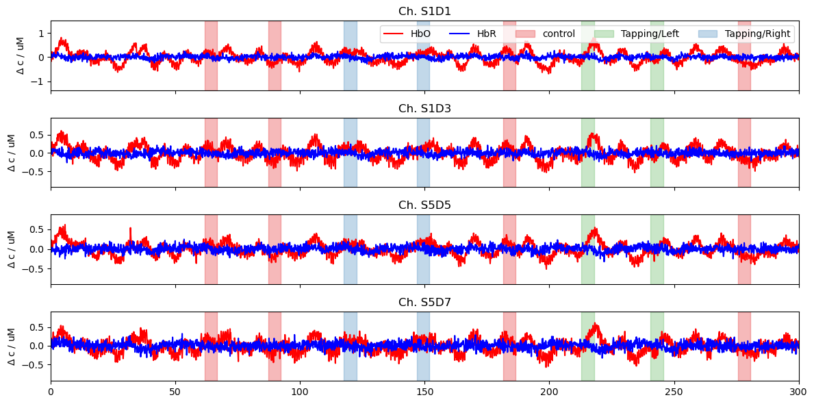
Now, we plot the frequnecy filtered concentration data for two channels from both the left (S1D1, S1D3) and right (S5D5, S5D7) hemispheres.
[4]:
ts = rec["conc_filtered"]

f, ax = p.subplots(4, 1, sharex=True, figsize=(12, 6))
for i, ch in enumerate(["S1D1", "S1D3", "S5D5", "S5D7"]):
    ax[i].plot(ts.time, ts.sel(channel=ch, chromo="HbO"), "r-", label="HbO")
    ax[i].plot(ts.time, ts.sel(channel=ch, chromo="HbR"), "b-", label="HbR")
    ax[i].set_title(f"Ch. {ch}")
    vbx.plot_stim_markers(ax[i], rec.stim, y=1)
    ax[i].set_ylabel(r"$\Delta$ c / uM")

ax[0].legend(ncol=6)
ax[3].set_label("time / s")
ax[3].set_xlim(0,300)
p.tight_layout()
Build design matrix
We can build a design matrix by concatenating different regressors. The regressor functions are found in glm.design_matrix. A regressor or sum of regressors returns a DesignMatrix object with two attributes:
common (xr.DataArray): regressors that apply to all channels, e.g. - HRF regressors - drift regressors - constant term
channel_wise (list[xr.DataArray]): regressors that can differ between channels, such as short-distance channel regressors.
In this example, we use short-distance channel regression to account for signal components from superficial layers: for each long channel the closest short channel is selected. From these the channel-wise regressor ‘short’ is derived.
The regressor function closest_short_channel_regressor requires the following arguments:
ts_long: Time series of long channels
ts_short: Time series of short channels
geo3d: Probe geometry
We use the utility function nirs.split_long_short_channels to create the two distance-based timeseries ts_long and ts_short.
[5]:
# split time series into two based on channel distance
ts_long, ts_short = cedalion.nirs.split_long_short_channels(
    rec["conc_filtered"], rec.geo3d, distance_threshold=1.5 * units.cm
)

# create design matrix from hrf and short channel regressors
dms = (
    glm.design_matrix.hrf_regressors(
        ts_long, rec.stim, glm.Gamma(tau=0 * units.s, sigma=3 * units.s)
    )
    & glm.design_matrix.closest_short_channel_regressor(ts_long, ts_short, rec.geo3d)
)
The design matrix dms.common holds all regressors that apply to all channels. It has dimensions ‘time’, ‘chromo’ and ‘regressor’. Regressors have string labels.
[6]:
display(dms)
display(dms.common)
DesignMatrix(common=['HRF control','HRF Tapping/Left','HRF Tapping/Right'], channel_wise=['short'])
<xarray.DataArray (time: 23239, regressor: 3, chromo: 2)> Size: 1MB
0.0 0.0 0.0 0.0 0.0 0.0 0.0 0.0 0.0 0.0 ... 0.0 0.0 0.0 0.0 0.0 0.0 0.0 0.0 0.0
Coordinates:
  * time       (time) float64 186kB 0.0 0.128 0.256 ... 2.974e+03 2.974e+03
  * regressor  (regressor) <U17 204B 'HRF control' ... 'HRF Tapping/Right'
  * chromo     (chromo) <U3 24B 'HbO' 'HbR'
channel_wise_regressors is list of additional xr.DataArrays that contain regressors which differ between channels. Each such array may contain only one regressor (i.e. the size of the regressor dimension must be 1). The regressors for each channel are arranged in the additional ‘channel’ dimension.
[7]:
display(dms.channel_wise[0]) # list contains only one element (short channel regressor)

# normalize short channel regressor and remove units
dms.channel_wise[0] = dms.channel_wise[0].pint.dequantify()
dms.channel_wise[0] /= dms.channel_wise[0].max("time")
<xarray.DataArray 'concentration' (regressor: 1, chromo: 2, channel: 20,
                                   time: 23239)> Size: 7MB
[µM] -0.1671 -0.3522 -0.03758 0.1025 ... 0.06639 -0.001217 0.005855 -0.001648
Coordinates:
  * chromo         (chromo) <U3 24B 'HbO' 'HbR'
  * time           (time) float64 186kB 0.0 0.128 0.256 ... 2.974e+03 2.974e+03
    samples        (time) int64 186kB 0 1 2 3 4 ... 23235 23236 23237 23238
  * channel        (channel) object 160B 'S1D1' 'S1D2' 'S1D3' ... 'S8D7' 'S8D8'
    short_channel  (channel) object 160B 'S1D9' 'S1D9' ... 'S8D16' 'S8D16'
    comp_group     (channel) int64 160B 0 0 0 1 1 1 2 2 3 3 4 4 4 5 5 5 6 6 7 7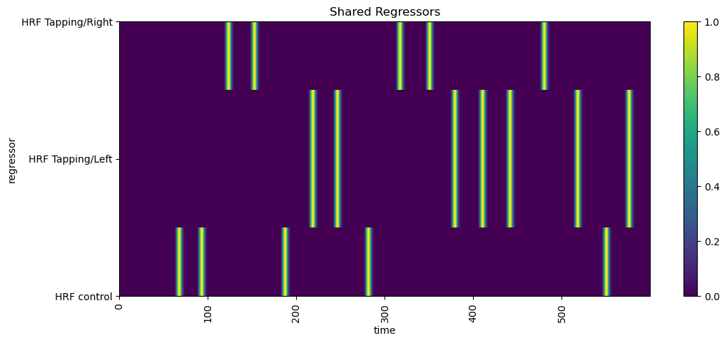
* regressor (regressor) <U5 20B 'short'Visualize the design matrix
First, we’ll plot the common regressors (those applying to all channels) using xr.DataArray.plot. This enables us to compare the onsets/offsets of each regressor.
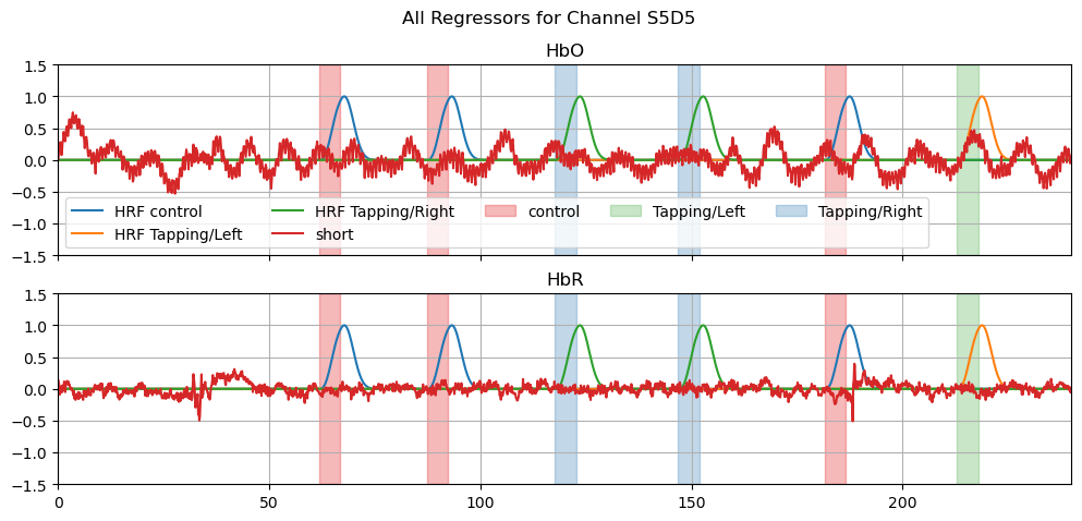
Next, we create a line plot of all regressors in the design matrix of one selected channel, including channel-wise regressors.
[8]:
# select common regressors
dm = dms.common
display(dm)

# using xr.DataArray.plot
f, ax = p.subplots(1,1,figsize=(12,5))
dm.sel(chromo="HbO", time=dm.time < 600).T.plot()
p.title("Shared Regressors")
p.xticks(rotation=90)
p.show()

# line plots of all regressors
f, ax = p.subplots(2,1,sharex=True, figsize=(12,5))

ch = "S5D5"

reg_colors = {"HRF control" : "r", "HRF Tapping/Left" : "g", "HRF Tapping/Right" : "b"}

for i, chromo in enumerate(["HbO", "HbR"]):
    for reg in dm.regressor.values:
        normed_reg = dm.sel(chromo=chromo, regressor=reg)
        normed_reg /= normed_reg.max()
        ax[i].plot(dm.time, normed_reg, label=reg, c=reg_colors[reg])

    for cwr in dms.channel_wise:
        for reg in cwr.regressor.values:
            normed_reg = cwr.sel(chromo=chromo, regressor=reg, channel=ch)
            normed_reg /= normed_reg.max()
            ax[i].plot(cwr.time, normed_reg, label=reg)
    vbx.plot_stim_markers(ax[i], rec.stim, y=1)
    ax[i].grid()
    ax[i].set_title(chromo)
    ax[i].set_ylim(-1.5,1.5)
f.suptitle("All Regressors for Channel " + ch)
ax[0].legend(ncol=5)
ax[0].set_xlim(0,240);
<xarray.DataArray (time: 23239, regressor: 3, chromo: 2)> Size: 1MB
0.0 0.0 0.0 0.0 0.0 0.0 0.0 0.0 0.0 0.0 ... 0.0 0.0 0.0 0.0 0.0 0.0 0.0 0.0 0.0
Coordinates:
  * time       (time) float64 186kB 0.0 0.128 0.256 ... 2.974e+03 2.974e+03
  * regressor  (regressor) <U17 204B 'HRF control' ... 'HRF Tapping/Right'
  * chromo     (chromo) <U3 24B 'HbO' 'HbR'
Fitting the model
The method glm.fit is used to fit the GLM to the time series. The required arguments are timeseries and design matrix. We can optionally specify the noise model from the following currently available options:
ols (default): ordinary least squares
rls: recursive least squares
wls: weighted least squares
ar_irls: autoregressive iteratively reweighted least squares [BAH13]
gls: generalized least squares
glsar: generalized least squares with autoregressive covariance structure
The fit method returns an xr.DataArray of statsmodels RegressionResults objects with dimensions (channel, chromo). Any RegressionResults method can be called on this DataArray using the .sm accessor. For example, we access the betas or model coefficients by using result.sm.params. Please refer to the statsmodels documentation for a full list of methods and attributes.
[9]:
results = glm.fit(ts_long, dms, noise_model="ar_irls", max_jobs=1)

display(results)
<xarray.DataArray (channel: 20, chromo: 2)> Size: 320B
<statsmodels.robust.robust_linear_model.RLMResultsWrapper object at 0x7f62746...
Coordinates:
  * chromo    (chromo) <U3 24B 'HbO' 'HbR'
  * channel   (channel) object 160B 'S1D1' 'S1D2' 'S1D3' ... 'S8D7' 'S8D8'
    source    (channel) object 160B 'S1' 'S1' 'S1' 'S2' ... 'S7' 'S7' 'S8' 'S8'
    detector  (channel) object 160B 'D1' 'D2' 'D3' 'D1' ... 'D6' 'D7' 'D7' 'D8'
Attributes:
description: AR_IRLS[10]:
# access the fitted model parameters
betas = results.sm.params
display(betas)
display(betas.rename("betas").to_dataframe())
<xarray.DataArray (channel: 20, chromo: 2, regressor: 4)> Size: 1kB
-0.01868 0.2882 0.348 0.2294 -0.004345 ... -0.0007166 -0.01868 -0.02131 0.09559
Coordinates:
  * regressor  (regressor) object 32B 'HRF control' ... 'short'
  * chromo     (chromo) <U3 24B 'HbO' 'HbR'
  * channel    (channel) object 160B 'S1D1' 'S1D2' 'S1D3' ... 'S8D7' 'S8D8'
    source     (channel) object 160B 'S1' 'S1' 'S1' 'S2' ... 'S7' 'S7' 'S8' 'S8'
    detector   (channel) object 160B 'D1' 'D2' 'D3' 'D1' ... 'D6' 'D7' 'D7' 'D8'
Attributes:
description: AR_IRLS| source | detector | betas | |||
|---|---|---|---|---|---|
| channel | chromo | regressor | |||
| S1D1 | HbO | HRF control | S1 | D1 | -0.018679 |
| HRF Tapping/Left | S1 | D1 | 0.288181 | ||
| HRF Tapping/Right | S1 | D1 | 0.348023 | ||
| short | S1 | D1 | 0.229398 | ||
| HbR | HRF control | S1 | D1 | -0.004345 | |
| ... | ... | ... | ... | ... | ... |
| S8D8 | HbO | short | S8 | D8 | 1.398041 |
| HbR | HRF control | S8 | D8 | -0.000717 | |
| HRF Tapping/Left | S8 | D8 | -0.018676 | ||
| HRF Tapping/Right | S8 | D8 | -0.021308 | ||
| short | S8 | D8 | 0.095589 |
160 rows × 3 columns
The statsmodels integration gives useful information about the uncertainty of our GLM fit. For example, here we calculate the confidence interval for the betas associated with channel S1D1.
[11]:
# best fit parameters + confidence intervals
s1d1_conf_int = results[0,0].item().conf_int()
s1d1_conf_int.columns = ["Confidence Interval Lower", "Confidence Interval Upper"]
s1d1_betas = results[0,0].item().params.rename("betas_S1D1")
df = pd.concat([s1d1_conf_int, s1d1_betas], axis=1)
df = df[["Confidence Interval Lower", "betas_S1D1", "Confidence Interval Upper"]]
display(df)
| Confidence Interval Lower | betas_S1D1 | Confidence Interval Upper | |
|---|---|---|---|
| HRF control | -0.059929 | -0.018679 | 0.022571 |
| HRF Tapping/Left | 0.246885 | 0.288181 | 0.329477 |
| HRF Tapping/Right | 0.306695 | 0.348023 | 0.389351 |
| short | 0.219608 | 0.229398 | 0.239187 |
Model Predictions
Using glm.predict one can scale the regressors in dm and channel_wise_regressors with the estimated coefficients to obtain a model prediction. By giving only a subset of betas to glm.predict one can predict subcomponents of the model. For example, this is useful when we want to separate HRF from drift components in our model.
[12]:
# prediction using all regressors
betas = results.sm.params
pred = glm.predict(ts_long, betas, dms)#, channel_wise_regressors)

# prediction of all nuisance regressors, i.e. all regressors that don't start with 'HRF '
pred_wo_hrf = glm.predict(
    ts_long,
    betas.sel(regressor=~betas.regressor.str.startswith("HRF ")),
    dms,
)

# prediction of all HRF regressors, i.e. all regressors that start with 'HRF '
pred_hrf = glm.predict(
    ts_long,
    betas.sel(regressor=betas.regressor.str.startswith("HRF ")),
    dms,
)
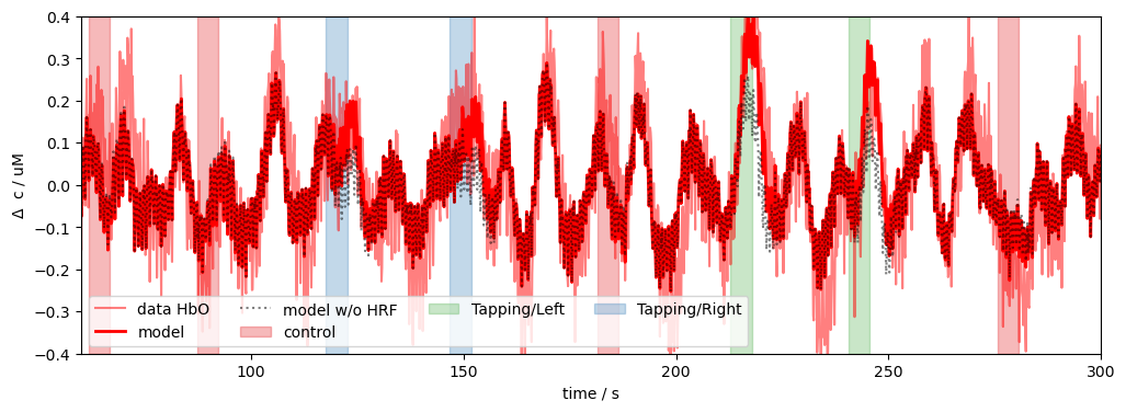
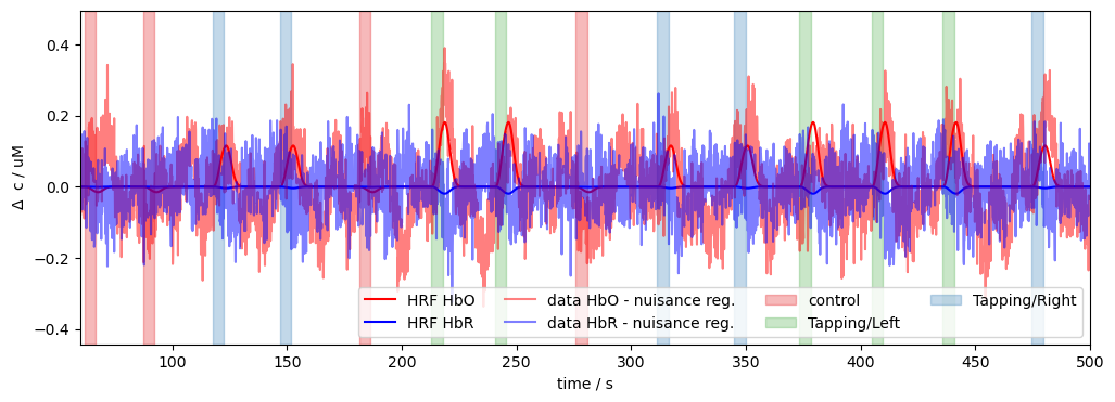
Plot model predictions
Now, we’ll plot our model prediction for a single channel. In order to visualize the distinct contributions of different regressors, we plot the predictions of different groups of regressors (all, w/o HRF, only HRF).
[13]:
# plot the data and model prediction
ch = "S5D5"
f, ax = p.subplots(1,1, figsize=(12, 4))
p.plot(ts_long.time, ts_long.sel(chromo="HbO", channel=ch), "r-", label="data HbO", alpha=.5)
p.plot(pred.time, pred.sel(chromo="HbO", channel=ch), "r-", label="model", lw=2 )
p.plot(pred.time, pred_wo_hrf.sel(chromo="HbO", channel=ch), "k:", label="model w/o HRF", alpha=.5)
vbx.plot_stim_markers(ax, rec.stim, y=1)
p.xlim(60,300)
p.ylim(-.4,.4)
p.xlabel("time / s")
p.ylabel(r"$\Delta$  c / uM")
p.legend(ncol=4)


# subtract nuisance regressors from data and plot against predicted HRF components
f, ax = p.subplots(1,1, figsize=(12, 4))
p.plot(pred_hrf.time, pred_hrf.sel(chromo="HbO", channel=ch), "r-", label="HRF HbO")
p.plot(pred_hrf.time, pred_hrf.sel(chromo="HbR", channel=ch), "b-", label="HRF HbR")
p.plot(
    pred_hrf.time,
    ts_long.sel(chromo="HbO", channel=ch).pint.dequantify() - pred_wo_hrf.sel(chromo="HbO", channel=ch),
    "r-", label="data HbO - nuisance reg.", alpha=.5
)
p.plot(
    pred_hrf.time,
    ts_long.sel(chromo="HbR", channel=ch).pint.dequantify() - pred_wo_hrf.sel(chromo="HbR", channel=ch),
    "b-", label="data HbR - nuisance reg.", alpha=.5
)
vbx.plot_stim_markers(ax, rec.stim, y=1)
p.legend(ncol=4, loc="lower right")

p.xlim(60,500)
p.xlabel("time / s")
p.ylabel(r"$\Delta$  c / uM");
Scalp plots
In this section of the notebook, we visualize our GLM using cedalion’s scalp plotting functionality. See the cedalion API documentation for more information on the plots.scalp_plot function.
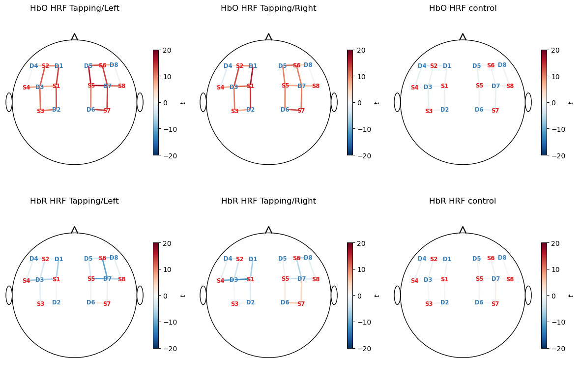
Betas
First, we visualize the coefficient values of our GLM.
[14]:
f, ax = p.subplots(2, 3, figsize=(12, 8))
vlims = {"HbO" : [-0.015,0.015], "HbR" : [-0.003, 0.003]}
for i_chr, chromo in enumerate(betas.chromo.values):
    vmin, vmax = vlims[chromo]
    for i_reg, reg in enumerate(
        ["HRF Tapping/Left", "HRF Tapping/Right", "HRF control"]
    ):
        cedalion.vis.anatomy.scalp_plot(
            rec["amp"],
            rec.geo3d,
            betas.sel(chromo=chromo, regressor=reg),
            ax[i_chr, i_reg],
            min_dist=1.5 * cedalion.units.cm,
            title=f"{chromo} {reg}",
            vmin=vmin,
            vmax=vmax,
            optode_labels=True,
            cmap="RdBu_r",
            cb_label=r"$\beta$"
        )
p.tight_layout()
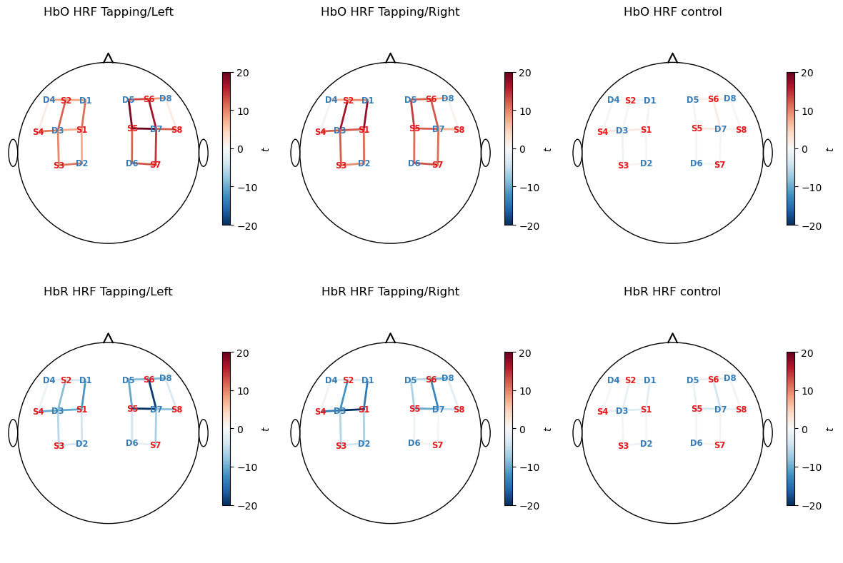
T-Values
Now, we will calculate t-values for our model coefficients and display them on a scalp plot.
[15]:
display(results.sm.tvalues)
results.sm.tvalues.min().item(), results.sm.tvalues.max().item() # min and max t-values across all regressors
<xarray.DataArray (channel: 20, chromo: 2, regressor: 4)> Size: 1kB
-0.8875 13.68 16.5 45.93 -0.6809 -6.457 ... 238.1 -0.05769 -1.503 -1.715 26.78
Coordinates:
  * regressor  (regressor) object 32B 'HRF control' ... 'short'
  * chromo     (chromo) <U3 24B 'HbO' 'HbR'
  * channel    (channel) object 160B 'S1D1' 'S1D2' 'S1D3' ... 'S8D7' 'S8D8'
    source     (channel) object 160B 'S1' 'S1' 'S1' 'S2' ... 'S7' 'S7' 'S8' 'S8'
    detector   (channel) object 160B 'D1' 'D2' 'D3' 'D1' ... 'D6' 'D7' 'D7' 'D8'
Attributes:
description: AR_IRLS[15]:
(-12.327211754370465, 251.26199966682327)
[16]:
# plot t-values of fitted model parameters
f, ax = p.subplots(2, 3, figsize=(12, 8))
vlims = {"HbO" : [-20,20], "HbR" : [-20, 20]}
for i_chr, chromo in enumerate(betas.chromo.values):
    vmin, vmax = vlims[chromo]
    for i_reg, reg in enumerate(["HRF Tapping/Left", "HRF Tapping/Right", "HRF control"]):
        cedalion.vis.anatomy.scalp_plot(
            rec["amp"],
            rec.geo3d,
            results.sm.tvalues.sel(chromo=chromo, regressor=reg),
            ax[i_chr, i_reg],
            min_dist=1.5 * cedalion.units.cm,
            title=f"{chromo} {reg}",
            vmin=vmin,
            vmax=vmax,
            optode_labels=True,
            cmap="RdBu_r",
            cb_label=r"$t$"
        )
p.tight_layout()
References
[17]:
cedalion.bib.dump_to_notebook()
Methods used
| [1] | Luke2021 | cedalion.data.get_fingertapping | Robert Luke and David McAlpine. fNIRS Finger Tapping Data in BIDS Format. September 2021. doi:10.5281/zenodo.5529797. |
| [2] | Tucker2022 | cedalion.io.snirf.read_snirf | Stephen Tucker, Jay Dubb, Sreekanth Kura, Alexander von Lühmann, Robert Franke, Jörn M. Horschig, Samuel Powell, Robert Oostenveld, Michael Lührs, Édouard Delaire, Zahra M. Aghajan, Hanseok Yun, Meryem A. Yücel, Qianqian Fang, Theodore J. Huppert, Blaise deB. Frederick, Luca Pollonini, David A. Boas, and Robert Luke. Introduction to the shared near infrared spectroscopy format. Neurophotonics, 10(1):013507, 2022. doi:10.1117/1.NPh.10.1.013507. |
| [3] | Delpy1988 | cedalion.nirs.cw.int2od, cedalion.nirs.cw.od2conc | D. T. Delpy, M. Cope, P. van der Zee, S. Arridge, S. Wray, and J. Wyatt. Estimation of optical pathlength through tissue from direct time of flight measurement. Physics in Medicine and Biology, 33(12):1433–1442, 1988. doi:10.1088/0031-9155/33/12/008. |
| [4] | Villringer1997 | cedalion.nirs.cw.int2od, cedalion.nirs.cw.od2conc | Arno Villringer and Britton Chance. Non-invasive optical spectroscopy and imaging of human brain function. Trends in Neurosciences, 20(10):435–442, 1997. doi:10.1016/S0166-2236(97)01132-6. |
| [5] | Prahl1998 | cedalion.nirs.common.get_extinction_coefficients | Scott A. Prahl. Optical absorption of hemoglobin. Oregon Medical Laser Center, online resource, 1998. URL: https://omlc.org/spectra/hemoglobin/. |
| [6] | Strangman2002 | cedalion.models.glm.basis_functions.Gamma.__call__ | Gary Strangman, Joseph P. Culver, John H. Thompson, and David A. Boas. A quantitative comparison of simultaneous BOLD fMRI and NIRS recordings during functional brain activation. NeuroImage, 17(2):719–731, 2002. doi:10.1006/nimg.2002.1227. |
| [7] | Huppert2009 | cedalion.models.glm.design_matrix.closest_short_channel_regressor | Theodore J. Huppert, Solomon G. Diamond, Maria A. Franceschini, and David A. Boas. Homer: a review of time-series analysis methods for near-infrared spectroscopy of the brain. Appl. Opt., 48(10):D280–D298, Apr 2009. doi:https://doi.org/10.1364/AO.48.00D280. |
| [8] | Barker2013 | cedalion.math.ar_irls.ar_irls_GLM, cedalion.models.glm.solve.fit | Jeffrey W. Barker, Ardalan Aarabi, and Theodore J. Huppert. Autoregressive model based algorithm for correcting motion and serially correlated errors in fnirs. Biomed. Opt. Express, 4(8):1366–1379, Aug 2013. doi:10.1364/BOE.4.001366. |