Synthetic Artifacts
[1]:
# This cells setups the environment when executed in Google Colab.
try:
    import google.colab
    !curl -s https://raw.githubusercontent.com/ibs-lab/cedalion/dev/scripts/colab_setup.py -o colab_setup.py
    # Select branch with --branch "branch name" (default is "dev")
    %run colab_setup.py
except ImportError:
    pass
[2]:
import matplotlib.pyplot as p
import xarray as xr

import cedalion
import cedalion.data as data
import cedalion.nirs
import cedalion.sim.synthetic_artifact as sa
First, we’ll load some example data.
[3]:
rec = data.get_fingertapping()
rec["od"] = cedalion.nirs.cw.int2od(rec["amp"])

f, ax = p.subplots(1, 1, figsize=(12, 4))
ax.plot(
    rec["amp"].time,
    rec["amp"].sel(channel="S3D3", wavelength="850"),
    "g-",
    label="850nm",
)
ax.plot(
    rec["amp"].time,
    rec["amp"].sel(channel="S3D3", wavelength="760"),
    "r-",
    label="760nm",
)
p.legend()
ax.set_xlabel("time / s")
ax.set_ylabel("intensity / v")

display(rec["od"])
<xarray.DataArray (channel: 28, wavelength: 2, time: 23239)> Size: 10MB
<Quantity([[[ 0.04042072  0.04460046  0.04421587 ...  0.01087635  0.01189059
    0.00684764]
  [ 0.0238205   0.02007699  0.03480909 ...  0.02399285  0.02704088
    0.03173299]]

 [[-0.00828006 -0.01784406 -0.00219874 ... -0.00359206 -0.00674273
   -0.0047444 ]
  [-0.03725579 -0.04067296 -0.02826115 ...  0.00827539  0.00577114
    0.00515152]]

 [[ 0.10055823  0.09914287  0.11119026 ... -0.02830701 -0.02324277
   -0.02359042]
  [ 0.049938    0.04755176  0.06016311 ... -0.00545623 -0.00153089
   -0.00473309]]

 ...

 [[ 0.0954341   0.11098679  0.10684828 ... -0.03859972 -0.03566192
   -0.04378948]
  [ 0.03858011  0.06286433  0.0612825  ...  0.0083141   0.00767436
   -0.00267514]]

 [[ 0.1550658   0.17214468  0.16880747 ... -0.06854981 -0.06838218
   -0.07333574]
  [ 0.10250045  0.12616269  0.12619078 ... -0.04061104 -0.04037113
   -0.0475059 ]]

 [[ 0.05805322  0.06125157  0.06083507 ... -0.0191578  -0.01900317
   -0.02034392]
  [ 0.02437702  0.03088664  0.03219055 ... -0.01108594 -0.01093651
   -0.01316727]]], 'dimensionless')>
Coordinates:
  * time        (time) float64 186kB 0.0 0.128 0.256 ... 2.974e+03 2.974e+03
    samples     (time) int64 186kB 0 1 2 3 4 5 ... 23234 23235 23236 23237 23238
  * channel     (channel) object 224B 'S1D1' 'S1D2' 'S1D3' ... 'S8D8' 'S8D16'
    source      (channel) object 224B 'S1' 'S1' 'S1' 'S1' ... 'S8' 'S8' 'S8'
    detector    (channel) object 224B 'D1' 'D2' 'D3' 'D9' ... 'D7' 'D8' 'D16'
  * wavelength  (wavelength) float64 16B 760.0 850.0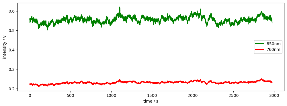
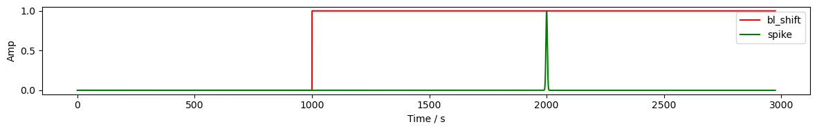
Artifact Generation
Artifacts are generated by functions taking as arguments:
time axis of timeseries
onset time
duration
To enable proper scaling, the amplitude of the generic artifact generated by these functions should be 1.
[4]:
time = rec["amp"].time

sample_bl_shift = sa.gen_bl_shift(time, 1000)
sample_spike = sa.gen_spike(time, 2000, 3)

display(sample_bl_shift)

fig, ax =  p.subplots(1, 1, figsize=(12,2))
ax.plot(time, sample_bl_shift, "r-", label="bl_shift")
ax.plot(time, sample_spike, "g-", label="spike")
ax.set_xlabel('Time / s')
ax.set_ylabel('Amp')
ax.legend()

p.tight_layout()
p.show()
<xarray.DataArray 'time' (time: 23239)> Size: 186kB
array([0., 0., 0., ..., 1., 1., 1.], shape=(23239,))
Coordinates:
  * time     (time) float64 186kB 0.0 0.128 0.256 ... 2.974e+03 2.974e+03
Controlling Artifact Timing
Artifacts can be placed using a timing dataframe with columns onset_time, duration, trial_type, value, and channel (extends stim dataframe).
We can use the function add_event_timing to create and modify timing dataframes. The function allows precise control over each event.
The function sel_chans_by_opt allows us to select a list of channels by way of a list of optodes. This reflects the fact that motion artifacts usually stem from the motion of a specific optode or set of optodes, which in turn affects all related channels.
We can also use the functions random_events_num and random_events_perc to add random events to the dataframe—specifying either the number of events or the percentage of the timeseries duration, respectively.
[5]:
# Create a list of events in the format (onset, duration)
events = [(1000, 1), (2000, 1)]

# Creates a new timing dataframe with the specified events.
# Setting channel to None indicates that the artifact applies to all channels.
timing_amp = sa.add_event_timing(events, 'bl_shift', None)

# Select channels by optode
chans = sa.sel_chans_by_opt(["S1"], rec["od"])

# Add random events to the timing dataframe
timing_od = sa.random_events_perc(time, 0.01, ["spike"], chans)

display(timing_amp)
display(timing_od)
| onset | duration | trial_type | value | channel | |
|---|---|---|---|---|---|
| 0 | 1000 | 1 | bl_shift | 1 | None |
| 1 | 2000 | 1 | bl_shift | 1 | None |
| onset | duration | trial_type | value | channel | |
|---|---|---|---|---|---|
| 0 | 540.257096 | 0.177696 | spike | 1 | [S1D1, S1D2, S1D3, S1D9] |
| 1 | 2894.197766 | 0.140083 | spike | 1 | [S1D1, S1D2, S1D3, S1D9] |
| 2 | 1373.998704 | 0.352955 | spike | 1 | [S1D1, S1D2, S1D3, S1D9] |
| 3 | 2527.483802 | 0.359413 | spike | 1 | [S1D1, S1D2, S1D3, S1D9] |
| 4 | 614.151196 | 0.110804 | spike | 1 | [S1D1, S1D2, S1D3, S1D9] |
| ... | ... | ... | ... | ... | ... |
| 112 | 480.162767 | 0.399272 | spike | 1 | [S1D1, S1D2, S1D3, S1D9] |
| 113 | 737.593897 | 0.245472 | spike | 1 | [S1D1, S1D2, S1D3, S1D9] |
| 114 | 2783.556565 | 0.265363 | spike | 1 | [S1D1, S1D2, S1D3, S1D9] |
| 115 | 2428.551448 | 0.330927 | spike | 1 | [S1D1, S1D2, S1D3, S1D9] |
| 116 | 150.815708 | 0.371829 | spike | 1 | [S1D1, S1D2, S1D3, S1D9] |
117 rows × 5 columns
Adding Artifacts to Data
The function add_artifacts automatically scales artifacts and adds them to timeseries data. The function takes arguments
ts: cdt.NDTimeSeries
timing: pd.DataFrame
artifacts: Dict
(mode): ‘auto’ (default) or ‘manual’
(scale): float = 1
(window_size): float = 120s
The artifact functions (see above) are passed as a dictionary. Keys correspond to entries in the column trial_type of the timing dataframe, i.e. each event specified in the timing dataframe is generated using the function artifacts[trial_type]. If mode is ‘manual’, artifacts are scaled directly by the scale parameter, otherwise artifacts are automatically scaled by a parameter alpha which is calculated using a sliding window approach.
If we want to auto scale based on concentration amplitudes but to add the artifacts to OD data, we can use the function add_chromo_artifacts_2_od. The function requires slightly different arguments because of the conversion between OD and conc:
ts: cdt.NDTimeSeries
timing: pd.DataFrame
artifacts: Dict
dpf: differential pathlength factor
geo3d: geometry of optodes (see recording object description)
(scale)
(window_size)
[6]:
artifacts = {"spike": sa.gen_spike, "bl_shift": sa.gen_bl_shift}

# Add baseline shifts to the amp data
rec["amp2"] = sa.add_artifacts(rec["amp"], timing_amp, artifacts)

# Convert the amp data to optical density
rec["od2"] = cedalion.nirs.cw.int2od(rec["amp2"])

dpf = xr.DataArray(
    [6, 6],
    dims="wavelength",
    coords={"wavelength": rec["amp"].wavelength},
)

# add spikes to od based on conc amplitudes
rec["od2"] = sa.add_chromo_artifacts_2_od(
    rec["od2"], timing_od, artifacts, rec.geo3d, dpf, 1.5
)

# Plot the OD data
channels = rec["od"].channel.values[0:6]
fig, axes = p.subplots(len(channels), 1, figsize=(12, len(channels) * 2))
if len(channels) == 1:
    axes = [axes]
for i, channel in enumerate(channels):
    ax = axes[i]
    ax.plot(
        rec["od2"].time,
        rec["od2"].sel(channel=channel, wavelength="850"),
        "g-",
        label="850nm + artifacts",
    )
    ax.plot(
        rec["od"].time,
        rec["od"].sel(channel=channel, wavelength="850"),
        "r-",
        label="850nm - od",
    )
    ax.set_title(f"Channel: {channel}")
    ax.set_xlabel("Time / s")
    ax.set_ylabel("OD")
    ax.legend()
p.tight_layout()
p.show()
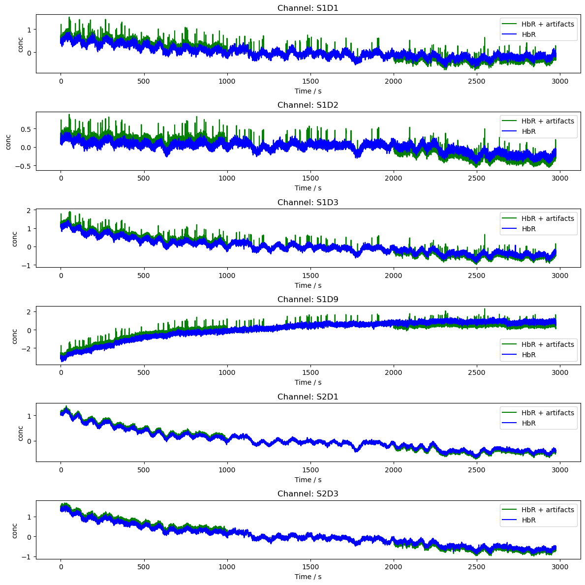
[7]:
# Plot the data in conc

rec["conc"] = cedalion.nirs.cw.od2conc(rec["od"], rec.geo3d, dpf)
rec["conc2"] = cedalion.nirs.cw.od2conc(rec["od2"], rec.geo3d, dpf)
channels = rec["od"].channel.values[0:6]
fig, axes = p.subplots(len(channels), 1, figsize=(12, len(channels) * 2))
if len(channels) == 1:
    axes = [axes]
for i, channel in enumerate(channels):
    ax = axes[i]
    ax.plot(
        rec["conc2"].time,
        rec["conc2"].sel(channel=channel, chromo="HbR"),
        "g-",
        label="HbR + artifacts",
    )
    ax.plot(
        rec["conc"].time,
        rec["conc"].sel(channel=channel, chromo="HbR"),
        "b-",
        label="HbR",
    )
    ax.set_title(f"Channel: {channel}")
    ax.set_xlabel("Time / s")
    ax.set_ylabel("conc")
    ax.legend()
p.tight_layout()
p.show()
Problems, improvements
One-function wrapper/interface?
More sophisticated artifacts (e.g. smooth baseline shift)
References
[8]:
cedalion.bib.dump_to_notebook()
Methods used
| [1] | Luke2021 | cedalion.data.get_fingertapping | Robert Luke and David McAlpine. fNIRS Finger Tapping Data in BIDS Format. September 2021. doi:10.5281/zenodo.5529797. |
| [2] | Tucker2022 | cedalion.io.snirf.read_snirf | Stephen Tucker, Jay Dubb, Sreekanth Kura, Alexander von Lühmann, Robert Franke, Jörn M. Horschig, Samuel Powell, Robert Oostenveld, Michael Lührs, Édouard Delaire, Zahra M. Aghajan, Hanseok Yun, Meryem A. Yücel, Qianqian Fang, Theodore J. Huppert, Blaise deB. Frederick, Luca Pollonini, David A. Boas, and Robert Luke. Introduction to the shared near infrared spectroscopy format. Neurophotonics, 10(1):013507, 2022. doi:10.1117/1.NPh.10.1.013507. |
| [3] | Delpy1988 | cedalion.nirs.cw.int2od, cedalion.nirs.cw.od2conc | D. T. Delpy, M. Cope, P. van der Zee, S. Arridge, S. Wray, and J. Wyatt. Estimation of optical pathlength through tissue from direct time of flight measurement. Physics in Medicine and Biology, 33(12):1433–1442, 1988. doi:10.1088/0031-9155/33/12/008. |
| [4] | Villringer1997 | cedalion.nirs.cw.int2od, cedalion.nirs.cw.od2conc | Arno Villringer and Britton Chance. Non-invasive optical spectroscopy and imaging of human brain function. Trends in Neurosciences, 20(10):435–442, 1997. doi:10.1016/S0166-2236(97)01132-6. |
| [5] | Prahl1998 | cedalion.nirs.common.get_extinction_coefficients | Scott A. Prahl. Optical absorption of hemoglobin. Oregon Medical Laser Center, online resource, 1998. URL: https://omlc.org/spectra/hemoglobin/. |