S3: Signal Processing
This notebook demonstrates Cedalion’s capabilities to assess signal quality and correct motion artifacts.
Several signal quality metrics are implemented in the package cedalion.sigproc.quality. From these metrics boolean masks are created which indicate whether the quality of a given time point or segment is acceptable or not. By combining these boolean masks, complex selection criteria can be formulated.
Learning objectives
In this notebook you will learn to:
Apply a complete fNIRS preprocessing pipeline: quality assessment → OD conversion → motion correction → filtering → haemoglobin concentration
Compute and apply SCI and SNR quality masks to prune bad channels
Use TDDR and wavelet correction for motion artefacts
Understand how each preprocessing step changes the signal
[1]:
# This cells setups the environment when executed in Google Colab.
try:
    import google.colab
    !curl -s https://raw.githubusercontent.com/ibs-lab/cedalion/dev/scripts/colab_setup.py -o colab_setup.py
    # Select branch with --branch "branch name" (default is "dev")
    %run colab_setup.py
except ImportError:
    pass
[2]:
import cedalion
import cedalion.data
import cedalion.sigproc.motion as motion
import cedalion.sigproc.quality as quality
import cedalion.vis.anatomy
import cedalion.vis.blocks as vbx
import cedalion.vis.colors as colors
import matplotlib.pyplot as p
import numpy as np
import pandas as pd
import xarray as xr
from cedalion import units
from cedalion.vis.quality import plot_quality_mask

xr.set_options(display_expand_data=False)
[2]:
<xarray.core.options.set_options at 0x7fd48ec7d910>
Load Data
The example starts by loading an example datasets via cedalion.data:
[3]:
rec = cedalion.data.get_fingertappingDOT()
Recording Container
The Recording container carries time series and related objects through the program in ordered dictionaries.
The dataset contains a single time series of fNIRS raw amplitudes. This is stored in the attribute rec.timeseries with key 'amp':
[4]:
rec.timeseries.keys()
[4]:
odict_keys(['amp'])
Among the data stored in the Recordingcontainer, the time series are access most frequently. Therefore, a shortcut is provided. The user can access items in .timeseries directly on the Recording container:
[5]:
rec["amp"] is rec.timeseries["amp"]
[5]:
True
Next to the fNIRS time series, the dataset contains also time series data from auxiliary sensors which are stored in .aux_ts:
[6]:
rec.aux_ts.keys()
[6]:
odict_keys(['ACCEL_X_1', 'ACCEL_Y_1', 'ACCEL_Z_1', 'GYRO_X_1', 'GYRO_Y_1', 'GYRO_Z_1', 'ExGa1', 'ExGa2', 'ExGa3', 'ExGa4', 'ECG', 'Respiration', 'PPG', 'SpO2', 'Heartrate', 'GSR', 'Temperature'])
Information about stimulus events is stored in a pandas.DataFrame under .stim. For each stimulus event the onset and duration is stored in seconds. Each event also includes a value indicating stimulus strength (e.g., the loudness of an auditory stimulus), which can be used to scale the amplitude of the modeled hemodynamic response. Finally, the trial type string label allows distinguishing different event types.
[7]:
rec.stim
[7]:
| onset | duration | value | trial_type | |
|---|---|---|---|---|
| 0 | 23.855104 | 10.0 | 1.0 | 1 |
| 1 | 54.132736 | 10.0 | 1.0 | 1 |
| 2 | 84.410368 | 10.0 | 1.0 | 1 |
| 3 | 114.688000 | 10.0 | 1.0 | 1 |
| 4 | 146.112512 | 10.0 | 1.0 | 1 |
| ... | ... | ... | ... | ... |
| 125 | 1431.535616 | 10.0 | 1.0 | 5 |
| 126 | 1526.038528 | 10.0 | 1.0 | 5 |
| 127 | 1650.819072 | 10.0 | 1.0 | 5 |
| 128 | 1805.418496 | 10.0 | 1.0 | 5 |
| 129 | 1931.116544 | 10.0 | 1.0 | 5 |
130 rows × 4 columns
When loading SNIRF files, trial types are derived from numeric stimulus markers. Cedalion registers the accessor .cd on DataFrames through which the user can modify stimulus dataframes. In the following the function .cd.rename_events is used to translate the numeric stimulus markers into descriptive names.
Users are free to choose any labels, but a consistent naming scheme is recommended because it makes selecting events easier. The dataset contains two motor tasks: finger tapping and ball squeezing executed both with the left and right hand:
[8]:
rec.stim.cd.rename_events(
    {
        "1": "Rest",
        "2": "FTapping/Left",
        "3": "FTapping/Right",
        "4": "BallSqueezing/Left",
        "5": "BallSqueezing/Right",
    }
)

rec.stim
[8]:
| onset | duration | value | trial_type | |
|---|---|---|---|---|
| 0 | 23.855104 | 10.0 | 1.0 | Rest |
| 1 | 54.132736 | 10.0 | 1.0 | Rest |
| 2 | 84.410368 | 10.0 | 1.0 | Rest |
| 3 | 114.688000 | 10.0 | 1.0 | Rest |
| 4 | 146.112512 | 10.0 | 1.0 | Rest |
| ... | ... | ... | ... | ... |
| 125 | 1431.535616 | 10.0 | 1.0 | BallSqueezing/Right |
| 126 | 1526.038528 | 10.0 | 1.0 | BallSqueezing/Right |
| 127 | 1650.819072 | 10.0 | 1.0 | BallSqueezing/Right |
| 128 | 1805.418496 | 10.0 | 1.0 | BallSqueezing/Right |
| 129 | 1931.116544 | 10.0 | 1.0 | BallSqueezing/Right |
130 rows × 4 columns
Selecting all BallSqueezing tasks:
[9]:
with pd.option_context("display.max_rows", 5):
    display(rec.stim[rec.stim.trial_type.str.startswith("BallSqueezing")])
| onset | duration | value | trial_type | |
|---|---|---|---|---|
| 97 | 8.486912 | 10.0 | 1.0 | BallSqueezing/Left |
| 98 | 161.021952 | 10.0 | 1.0 | BallSqueezing/Left |
| ... | ... | ... | ... | ... |
| 128 | 1805.418496 | 10.0 | 1.0 | BallSqueezing/Right |
| 129 | 1931.116544 | 10.0 | 1.0 | BallSqueezing/Right |
33 rows × 4 columns
Selecting all motor tasks with the left hand:
[10]:
with pd.option_context("display.max_rows", 5):
    display(rec.stim[rec.stim.trial_type.str.endswith("Left")])
| onset | duration | value | trial_type | |
|---|---|---|---|---|
| 65 | 99.549184 | 10.0 | 1.0 | FTapping/Left |
| 66 | 129.597440 | 10.0 | 1.0 | FTapping/Left |
| ... | ... | ... | ... | ... |
| 112 | 1962.541056 | 10.0 | 1.0 | BallSqueezing/Left |
| 113 | 1994.194944 | 10.0 | 1.0 | BallSqueezing/Left |
33 rows × 4 columns
Time Series
The 'amp' time series is represented as a xarray.DataArray with dimensions 'channel', 'wavelength' and 'time'. Three coordinate arrays are linked to the 'channel' dimension, specifying for each channel a string label as well as the string label and the corresponding source and detector labels (e.g. the first channel 'S1D1' is between source 'S1' and detector 'D1'). Coordinates of the 'wavelength' dimension indicate that this CW-fNIRS measurement was done
at 760 and 850 nm. The 'time' dimensions has timestamps and an absolute sample counter as coordinates.
The DataArray is quantified in units of Volts.
[11]:
rec["amp"]
[11]:
<xarray.DataArray (channel: 100, wavelength: 2, time: 8794)> Size: 14MB
[V] 0.0874 0.08735 0.08819 0.08887 0.0879 ... 0.09108 0.09037 0.09043 0.08999
Coordinates:
  * time        (time) float64 70kB 0.0 0.2294 0.4588 ... 2.017e+03 2.017e+03
    samples     (time) int64 70kB 0 1 2 3 4 5 ... 8788 8789 8790 8791 8792 8793
  * channel     (channel) object 800B 'S1D1' 'S1D2' 'S1D4' ... 'S14D31' 'S14D32'
    source      (channel) object 800B 'S1' 'S1' 'S1' 'S1' ... 'S14' 'S14' 'S14'
    detector    (channel) object 800B 'D1' 'D2' 'D4' 'D5' ... 'D29' 'D31' 'D32'
  * wavelength  (wavelength) float64 16B 760.0 850.0
Attributes:
data_type_group: unprocessed rawMontage
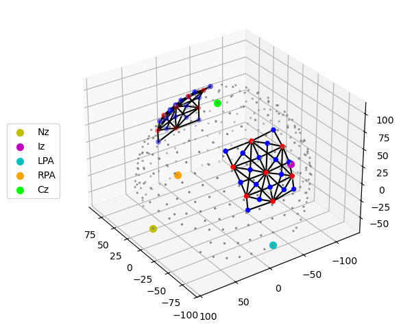
As described in the first tutorial, the probe geometry is stored in rec.geo3d as a DataArray of type cedalion.typing.LabeledPoints.
[12]:
rec.geo3d
[12]:
<xarray.DataArray (label: 346, digitized: 3)> Size: 8kB
[mm] -77.82 15.68 23.17 -61.91 21.23 56.49 ... 14.23 -38.28 81.95 -0.678 -37.03
Coordinates:
    type     (label) object 3kB PointType.SOURCE ... PointType.LANDMARK
  * label    (label) <U6 8kB 'S1' 'S2' 'S3' 'S4' ... 'FFT10h' 'FT10h' 'FTT10h'
Dimensions without coordinates: digitized[13]:
cedalion.vis.anatomy.plot_montage3D(rec["amp"], rec.geo3d)
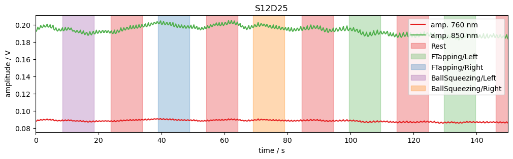
Using functions of matplotlib time trace for a single channel can be plotted. Note, how the time series amp is indexed by label to select channel and wavelengths.
The package cedalion.vis.blocks (imported as vbx) provides visualizations building blocks, such as adding stimulus markers to a plot.
[14]:
# example time trace
amp = rec["amp"]
ch = "S12D25"
f, ax = p.subplots(1, 1, figsize=(12, 3))
ax.set_prop_cycle("color", cedalion.vis.colors.COLORBREWER_Q8)
ax.plot(amp.time, amp.sel(channel=ch, wavelength=760), label="amp. 760 nm")
ax.plot(amp.time, amp.sel(channel=ch, wavelength=850), label="amp. 850 nm")
vbx.plot_stim_markers(ax, rec.stim, y=1)
ax.set_xlabel("time / s")
ax.set_ylabel("amplitude / V")
ax.set_xlim(0, 150)
ax.legend(loc="upper right")
ax.set_title(ch);
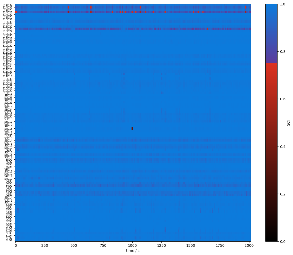
Quality Metrics : SCI & PSP
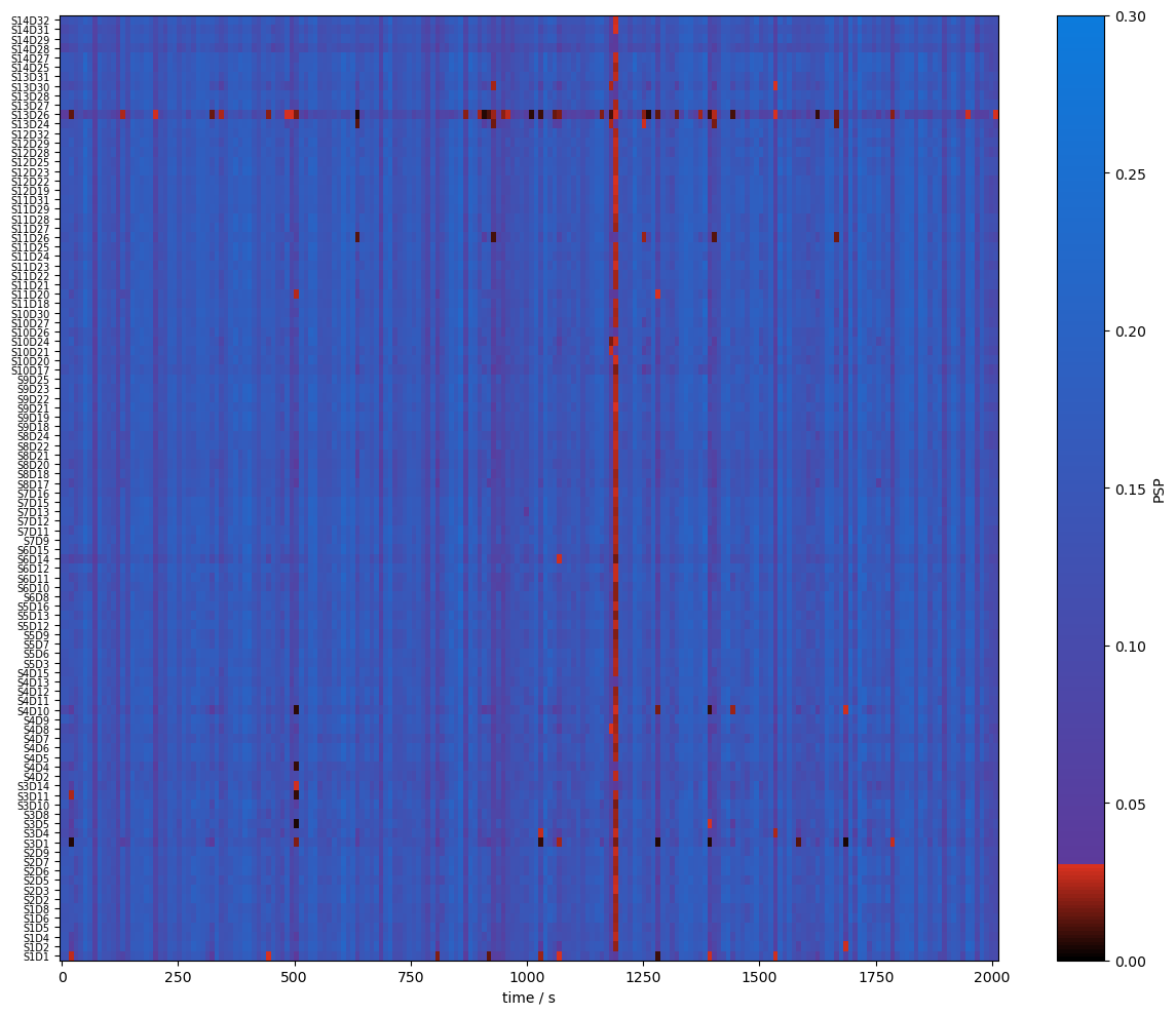
To assess the signal quality the Scalp Coupling Index (SCI) and Peak Spectral Power (PSP) are calculated with functions from cedalion.sigproc.quality. Both metrics are computed in 10-second sliding windows. Each metric a configurable threshold. Values exceeding the threshold indicate good signal quality. The functions sci and psp each return two DataArrays: one with the metric values, and one with a boolean mask indicating where the threshold is exceeded.
Since the metrics are calculated for each time window the time axis changed.
[15]:
sci_threshold = 0.75
window_length = 10 * units.s
sci, sci_mask = quality.sci(rec["amp"], window_length, sci_threshold)

psp_threshold = 0.03
psp, psp_mask = quality.psp(rec["amp"], window_length, psp_threshold)


display(sci.rename("sci"))
display(sci_mask.rename("sci_mask"))
<xarray.DataArray 'sci' (channel: 100, time: 200)> Size: 160kB
0.9949 0.9949 0.9775 0.9958 0.9914 0.9941 ... 0.9369 0.9498 0.9628 0.9718 0.9545
Coordinates:
  * time      (time) float64 2kB 0.0 10.09 20.19 ... 1.998e+03 2.008e+03
    samples   (time) int64 2kB 0 44 88 132 176 220 ... 8580 8624 8668 8712 8756
  * channel   (channel) object 800B 'S1D1' 'S1D2' 'S1D4' ... 'S14D31' 'S14D32'
    source    (channel) object 800B 'S1' 'S1' 'S1' 'S1' ... 'S14' 'S14' 'S14'
detector (channel) object 800B 'D1' 'D2' 'D4' 'D5' ... 'D29' 'D31' 'D32'<xarray.DataArray 'sci_mask' (channel: 100, time: 200)> Size: 20kB
True True True True True True True True ... True True True True True True True
Coordinates:
* time (time) float64 2kB 0.0 10.09 20.19 ... 1.998e+03 2.008e+03
samples (time) int64 2kB 0 44 88 132 176 220 ... 8580 8624 8668 8712 8756
* channel (channel) object 800B 'S1D1' 'S1D2' 'S1D4' ... 'S14D31' 'S14D32'
source (channel) object 800B 'S1' 'S1' 'S1' 'S1' ... 'S14' 'S14' 'S14'
detector (channel) object 800B 'D1' 'D2' 'D4' 'D5' ... 'D29' 'D31' 'D32'Visualize the metrics and quality masks:
[16]:
# define three colomaps: redish below a threshold, blueish above
sci_norm, sci_cmap = colors.threshold_cmap("sci_cmap", 0.0, 1.0, sci_threshold)
psp_norm, psp_cmap = colors.threshold_cmap("psp_cmap", 0.0, 0.30, psp_threshold)


def plot_sci(sci):
    # plot the heatmap
    f, ax = p.subplots(1, 1, figsize=(12, 10))

    m = ax.pcolormesh(sci.time, np.arange(len(sci.channel)), sci, shading="nearest", cmap=sci_cmap, norm=sci_norm)
    cb = p.colorbar(m, ax=ax)
    cb.set_label("SCI")
    ax.set_xlabel("time / s")
    p.tight_layout()
    ax.yaxis.set_ticks(np.arange(len(sci.channel)))
    ax.yaxis.set_ticklabels(sci.channel.values, fontsize=7)


def plot_psp(psp):
    f, ax = p.subplots(1, 1, figsize=(12, 10))

    m = ax.pcolormesh(psp.time, np.arange(len(psp.channel)), psp, shading="nearest", cmap=psp_cmap, norm=psp_norm)
    cb = p.colorbar(m, ax=ax)
    cb.set_label("PSP")
    ax.set_xlabel("time / s")
    p.tight_layout()
    ax.yaxis.set_ticks(np.arange(len(psp.channel)))
    ax.yaxis.set_ticklabels(psp.channel.values, fontsize=7)
[17]:
plot_sci(sci)
plot_quality_mask(sci > sci_threshold, f"SCI > {sci_threshold}")
plot_psp(psp)
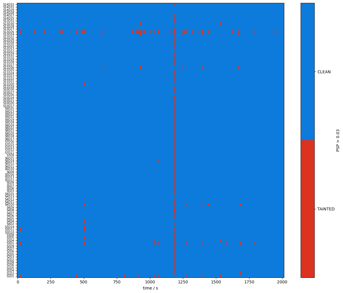
plot_quality_mask(psp > psp_threshold, f"PSP > {psp_threshold}")
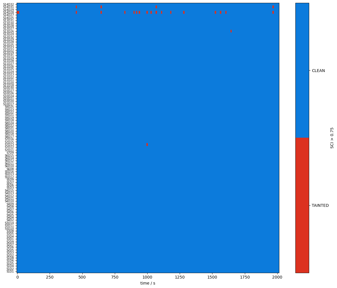
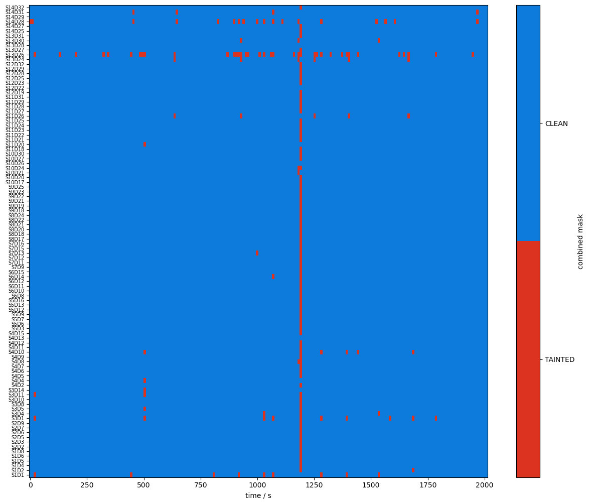
A window shall be considered clean only if both SCI and PSP exceed their respective thresholds. The user can combine the two boolean masks with a logical and, then compute the fraction of time windows where both conditions are true.
[18]:
combined_mask = sci_mask & psp_mask

display(combined_mask)
plot_quality_mask(combined_mask, "combined_mask")
<xarray.DataArray (channel: 100, time: 200)> Size: 20kB
True True False True True True True True ... True True True True True True True
Coordinates:
  * time      (time) float64 2kB 0.0 10.09 20.19 ... 1.998e+03 2.008e+03
    samples   (time) int64 2kB 0 44 88 132 176 220 ... 8580 8624 8668 8712 8756
  * channel   (channel) object 800B 'S1D1' 'S1D2' 'S1D4' ... 'S14D31' 'S14D32'
    source    (channel) object 800B 'S1' 'S1' 'S1' 'S1' ... 'S14' 'S14' 'S14'
    detector  (channel) object 800B 'D1' 'D2' 'D4' 'D5' ... 'D29' 'D31' 'D32'
The next cell calculates the percentage of clean time windows per channel. Afterwards, two channels are identified that are clean in fewer than 95% of the time windows.
[19]:
perc_time_clean = combined_mask.sum(dim="time") / len(sci.time)

display(perc_time_clean)

print("Channels clean less than 95% of the recording:")
display(perc_time_clean[perc_time_clean < 0.95])
<xarray.DataArray (channel: 100)> Size: 800B
0.955 0.99 0.995 0.995 0.995 0.995 0.995 ... 0.995 0.995 0.91 1.0 0.98 0.995
Coordinates:
  * channel   (channel) object 800B 'S1D1' 'S1D2' 'S1D4' ... 'S14D31' 'S14D32'
    source    (channel) object 800B 'S1' 'S1' 'S1' 'S1' ... 'S14' 'S14' 'S14'
    detector  (channel) object 800B 'D1' 'D2' 'D4' 'D5' ... 'D29' 'D31' 'D32'
Channels clean less than 95% of the recording:
<xarray.DataArray (channel: 2)> Size: 16B
0.815 0.91
Coordinates:
  * channel   (channel) object 16B 'S13D26' 'S14D28'
    source    (channel) object 16B 'S13' 'S14'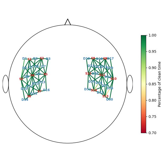
detector (channel) object 16B 'D26' 'D28'Visualize the percentage of clean times with a scalp plot:
[20]:
f, ax = p.subplots(1,1,figsize=(6.5,6.5))

cedalion.vis.anatomy.scalp_plot(
    rec["amp"],
    rec.geo3d,
    perc_time_clean,
    ax,
    cmap="RdYlGn",
    vmin=0.7,
    vmax=1,
    title=None,
    cb_label="Percentage of clean time",
    channel_lw=2,
    optode_labels=True
)
f.tight_layout()
Correct Motion Artifacts
Using the function cedalion.nirs.cw.int2od the raw amplitudes are converted to optical densities. Two motion-artifact correction methods are then applied.
First, Temporal Derivative Distribution Repair (TDDR) is used to repair unusually large jumps in the time series.
Second, a wavelet-based motion correction is applied.
The correction algorithms operate on optical densities. After correction, the corresponding corrected amplitudes are derived.
The modified time series are stored under different names in the Recording container.
[21]:
rec["od"] = cedalion.nirs.cw.int2od(rec["amp"])
rec["od_tddr"] = motion.tddr(rec["od"])
rec["od_wavelet"] = motion.wavelet(rec["od_tddr"])
rec["amp_corrected"] = cedalion.nirs.cw.od2int(
    rec["od_wavelet"], rec["amp"].mean("time")
)
Recalculate the SCI and PSP metrics on the corrected amplitudes and visualize the combined masks before and after correction.
[22]:
# recalculate sci & psp on cleaned data
sci_corr, sci_corr_mask = quality.sci(
    rec["amp_corrected"], window_length, sci_threshold
)
psp_corr, psp_corr_mask = quality.psp(
    rec["amp_corrected"], window_length, psp_threshold
)
combined_corr_mask = sci_corr_mask & psp_corr_mask
[23]:
plot_quality_mask(combined_mask, "combined mask")
plot_quality_mask(combined_corr_mask, "combined corrected mask")

Compare masks before and after motion artifact correction
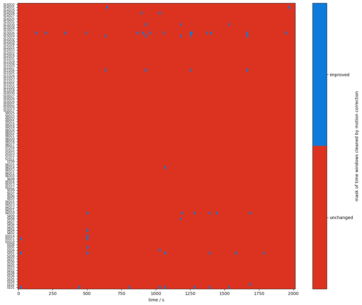
Using logical operations on the quality masks, the next cell identifies the time windows affected by the correction algorithms.
[24]:
changed_windows = (combined_mask == quality.TAINTED) & (combined_corr_mask == quality.CLEAN)

plot_quality_mask(
    changed_windows,
    "mask of time windows cleaned by motion correction",
    bool_labels=["unchanged", "improved"],
)

changed_windows = (combined_mask == quality.CLEAN) & (combined_corr_mask == quality.TAINTED)

plot_quality_mask(
    changed_windows,
    "mask of time windows corrupted by motion correction",
    bool_labels=["unchanged", "worsened"],
)

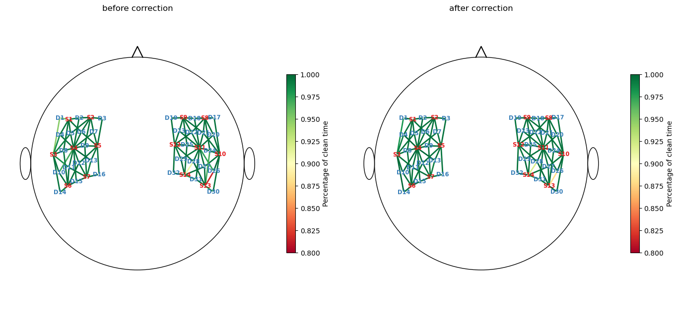
Recalculate and visualize the percentage of clean time:
[25]:
perc_time_clean_corr = combined_corr_mask.sum(dim="time") / len(sci.time)

f, ax = p.subplots(1,2,figsize=(14,6.5))

cedalion.vis.anatomy.scalp_plot(
    rec["amp"],
    rec.geo3d,
    perc_time_clean,
    ax[0],
    cmap="RdYlGn",
    vmin=0.80,
    vmax=1,
    title="before correction",
    cb_label="Percentage of clean time",
    channel_lw=2,
    optode_labels=True
)

cedalion.vis.anatomy.scalp_plot(
    rec["amp"],
    rec.geo3d,
    perc_time_clean_corr,
    ax[1],
    cmap="RdYlGn",
    vmin=0.80,
    vmax=1,
    title="after correction",
    cb_label="Percentage of clean time",
    channel_lw=2,
    optode_labels=True
)
f.tight_layout()
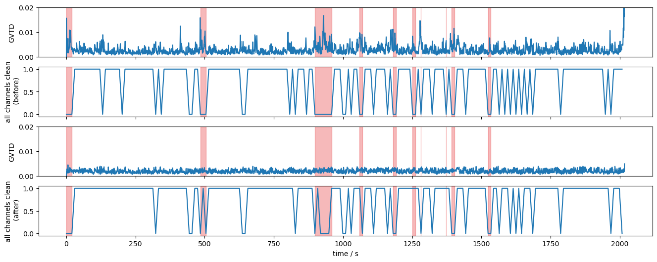
Global Variance of the Temporal Derivative (GVTD)
The GVTD metric allows identifying global bad time segments. Here, it is calculated for the original and corrected amplitudes.
[26]:
gvtd, gvtd_mask = quality.gvtd(rec["amp"])
gvtd_corr, gvtd_prr_mask = quality.gvtd(rec["amp_corrected"])
The 10 segments with highest GVTD values are selected:
[27]:
top10_bad_segments = sorted(
    [seg for seg in quality.mask_to_segments(combined_mask.all("channel"))],
    key=lambda t: gvtd.sel(time=slice(t[0], t[1])).max(),
    reverse=True,
)[:10]
The following plot shows the GVTD metric before and after corrections. The 10 selected segments are highlighted in red. The combined masks are further reduced to indicate, if all channels at a given time are clean.
The impact of the correction methods is evident in the reduced number of spikes in the GVTD trace and the improvements seen in the quality mask. Time windows that previously did not satisfy the all-channels-clean criteria meet it after correction.
[28]:
f,ax = p.subplots(4,1,figsize=(16,6), sharex=True)
ax[0].plot(gvtd.time, gvtd)
ax[1].plot(combined_mask.time, combined_mask.all("channel"))
ax[2].plot(gvtd_corr.time, gvtd_corr)
ax[3].plot(combined_corr_mask.time, combined_corr_mask.all("channel"))
ax[0].set_ylim(0, 0.02)
ax[2].set_ylim(0, 0.02)
ax[0].set_ylabel("GVTD")
ax[2].set_ylabel("GVTD")
ax[1].set_ylabel("all channels clean\n (before)")
ax[3].set_ylabel("all channels clean\n (after)")
ax[3].set_xlabel("time / s")

for i in range(4):
    vbx.plot_segments(ax[i], top10_bad_segments)
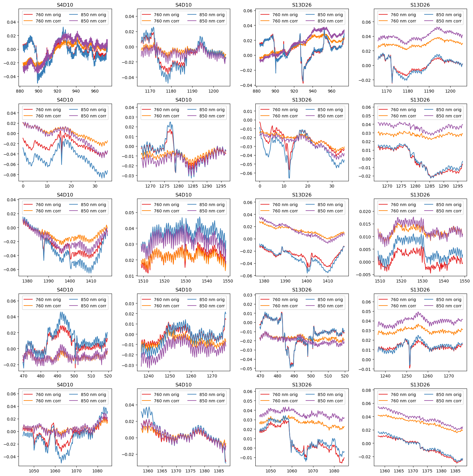
Visualize motion correction in selected segments
To illustrate the effect of TDDR and wavelet-based motion correction on the time series, the following cell plots the amplitudes for the ten selected segments in two channels before and after correction.
[29]:
example_channels = ["S4D10", "S13D26"]

f, ax = p.subplots(5,4, figsize=(16,16), sharex=False)
ax = ax.T.flatten()
padding = 15
i = 0
for ch in example_channels:
    for (start, end) in top10_bad_segments:
        ax[i].set_prop_cycle(color=["#e41a1c", "#ff7f00", "#377eb8", "#984ea3"])
        for wl in rec["od"].wavelength.values:
            sel = rec["od"].sel(time=slice(start-padding, end+padding), channel=ch, wavelength=wl)
            ax[i].plot(sel.time, sel, label=f"{wl:.0f} nm orig")
            sel = rec["od_wavelet"].sel(time=slice(start-padding, end+padding), channel=ch, wavelength=wl)
            ax[i].plot(sel.time, sel, label=f"{wl:.0f} nm corr")
            ax[i].set_title(ch)
        ax[i].legend(ncol=2, loc="upper center")
        ylim = ax[i].get_ylim()
        ax[i].set_ylim(ylim[0], ylim[1]+0.25*(ylim[1]-ylim[0])) # make space for legend

        i += 1

p.tight_layout()
Final channel selection
Before correction, the channels “S13D26” and “S14D28” had the most unclean time windows. Although the correction methods recovered some of these windows, the fraction of clean windows for both channels still remains below 95%.
[30]:
perc_time_clean_corr[perc_time_clean_corr < 0.95]
[30]:
<xarray.DataArray (channel: 2)> Size: 16B
0.88 0.92
Coordinates:
  * channel   (channel) object 16B 'S13D26' 'S14D28'
    source    (channel) object 16B 'S13' 'S14'
detector (channel) object 16B 'D26' 'D28'To prune bad channels from time series the function cedalion.sigproc.quality.prun_ch is available. It takes a list of quality masks, combines them and discards channels from the time series.
[31]:
signal_quality_selection_masks = [perc_time_clean >= .95]

rec["amp_pruned"], pruned_channels = quality.prune_ch(
    rec["amp"], signal_quality_selection_masks, "all"
)
display(rec["amp_pruned"])
display(pruned_channels)
<xarray.DataArray (channel: 98, wavelength: 2, time: 8794)> Size: 14MB
[V] 0.0874 0.08735 0.08819 0.08887 0.0879 ... 0.09108 0.09037 0.09043 0.08999
Coordinates:
  * time        (time) float64 70kB 0.0 0.2294 0.4588 ... 2.017e+03 2.017e+03
    samples     (time) int64 70kB 0 1 2 3 4 5 ... 8788 8789 8790 8791 8792 8793
  * channel     (channel) object 784B 'S1D1' 'S1D2' 'S1D4' ... 'S14D31' 'S14D32'
    source      (channel) object 784B 'S1' 'S1' 'S1' 'S1' ... 'S14' 'S14' 'S14'
    detector    (channel) object 784B 'D1' 'D2' 'D4' 'D5' ... 'D29' 'D31' 'D32'
  * wavelength  (wavelength) float64 16B 760.0 850.0
Attributes:
    data_type_group:  unprocessed raw
array(['S13D26', 'S14D28'], dtype=object)
References
[32]:
cedalion.bib.dump_to_notebook()
Methods used
| [1] | Tucker2022 | cedalion.io.snirf.read_snirf | Stephen Tucker, Jay Dubb, Sreekanth Kura, Alexander von Lühmann, Robert Franke, Jörn M. Horschig, Samuel Powell, Robert Oostenveld, Michael Lührs, Édouard Delaire, Zahra M. Aghajan, Hanseok Yun, Meryem A. Yücel, Qianqian Fang, Theodore J. Huppert, Blaise deB. Frederick, Luca Pollonini, David A. Boas, and Robert Luke. Introduction to the shared near infrared spectroscopy format. Neurophotonics, 10(1):013507, 2022. doi:10.1117/1.NPh.10.1.013507. |
| [2] | Pollonini2014 | cedalion.sigproc.quality.psp, cedalion.sigproc.quality.sci | Luca Pollonini, Cristen Olds, Homer Abaya, Heather Bortfeld, Michael S. Beauchamp, and John S. Oghalai. Auditory cortex activation to natural speech and simulated cochlear implant speech measured with functional near-infrared spectroscopy. Hearing Research, 309:84–93, 2014. doi:https://doi.org/10.1016/j.heares.2013.11.007. |
| [3] | Pollonini2016 | cedalion.sigproc.quality.psp, cedalion.sigproc.quality.sci | Luca Pollonini, Heather Bortfeld, and John S. Oghalai. PHOEBE: a method for real time mapping of optodes-scalp coupling in functional near-infrared spectroscopy. Biomedical Optics Express, 7(12):5104, Dec 2016. doi:10.1364/BOE.7.005104. |
| [4] | Delpy1988 | cedalion.nirs.cw.int2od | D. T. Delpy, M. Cope, P. van der Zee, S. Arridge, S. Wray, and J. Wyatt. Estimation of optical pathlength through tissue from direct time of flight measurement. Physics in Medicine and Biology, 33(12):1433–1442, 1988. doi:10.1088/0031-9155/33/12/008. |
| [5] | Villringer1997 | cedalion.nirs.cw.int2od | Arno Villringer and Britton Chance. Non-invasive optical spectroscopy and imaging of human brain function. Trends in Neurosciences, 20(10):435–442, 1997. doi:10.1016/S0166-2236(97)01132-6. |
| [6] | Fishburn2019 | cedalion.sigproc.motion.tddr | Frank A. Fishburn, Ruth S. Ludlum, Chandan J. Vaidya, and Andrei V. Medvedev. Temporal derivative distribution repair (tddr): a motion correction method for fnirs. NeuroImage, 184:171–179, 2019. doi:https://doi.org/10.1016/j.neuroimage.2018.09.025. |
| [7] | Fishburn2018 | cedalion.sigproc.motion.tddr | Frank Fishburn. Tddr. 2018. URL: https://github.com/frankfishburn/TDDR/. |
| [8] | Molavi2012 | cedalion.sigproc.motion.wavelet | Behnam Molavi and Guy A Dumont. Wavelet-based motion artifact removal for functional near-infrared spectroscopy. Physiological Measurement, 33(2):259, 2012. doi:10.1088/0967-3334/33/2/259. |
| [9] | Huppert2009 | cedalion.sigproc.motion.wavelet | Theodore J. Huppert, Solomon G. Diamond, Maria A. Franceschini, and David A. Boas. Homer: a review of time-series analysis methods for near-infrared spectroscopy of the brain. Appl. Opt., 48(10):D280–D298, Apr 2009. doi:https://doi.org/10.1364/AO.48.00D280. |
| [10] | Sherafati2020 | cedalion.sigproc.quality._get_gvtd_threshold, cedalion.sigproc.quality.gvtd | Arefeh Sherafati, Abraham Z. Snyder, Adam T. Eggebrecht, Karla M. Bergonzi, Tracy M. Burns-Yocum, Heather M. Lugar, Silvina L. Ferradal, Amy Robichaux-Viehoever, Christopher D. Smyser, Ben J. Palanca, Tamara Hershey, and Joseph P. Culver. Global motion detection and censoring in high-density diffuse optical tomography. Human Brain Mapping, 41(14):4093–4112, 2020. doi:https://doi.org/10.1002/hbm.25111. |
Next: 4 — Model-driven Analysis — GLM-based HRF estimation.