Visualization Examples using Cedalion Plot Functions
This notebook will be continuously extended to enable an easy look up of visualization functions.
In each example cell, we un-necessarily re-import the plotting subpackages to clarify which of these are needed for the plots.
[1]:
# This cells setups the environment when executed in Google Colab.
try:
    import google.colab
    !curl -s https://raw.githubusercontent.com/ibs-lab/cedalion/dev/scripts/colab_setup.py -o colab_setup.py
    # Select branch with --branch "branch name" (default is "dev")
    %run colab_setup.py
except ImportError:
    pass
Importing Packages
3rd party plotting packages
Most of Cedalion’s plotting functionality is based on Matplotlib and Pyvista packages
[2]:
import pyvista as pv
import matplotlib.pyplot as p
from IPython.display import Image

#pv.set_jupyter_backend('server') # this enables interactive plots
pv.set_jupyter_backend('static') # this enables static rendering
Other packages that will be used in this notebook
Dependencies for data processing
[3]:
import matplotlib.pyplot as plt
import numpy as np
import xarray as xr

import cedalion
import cedalion.data
import cedalion.dot as dot
import cedalion.io
import cedalion.nirs
import cedalion.sigproc.quality
import cedalion.dataclasses as cdc
import cedalion.xrutils as xrutils
from cedalion.io.forward_model import FluenceFile
Load Data for Visuatization
This cell fetches a variety example datasets from the cloud for visualization. This can take a bit of time.
[4]:
# Loads a high-density finger tapping dataset into a recording container
rec = cedalion.data.get_fingertappingDOT()

# Loads a photogrammetric example scan
fname_scan, fname_snirf, fname_montage = cedalion.data.get_photogrammetry_example_scan()
pscan = cedalion.io.read_einstar_obj(fname_scan)

# Loads a precalculated example fluence profile
fluence_fname = cedalion.data.get_precomputed_fluence("fingertappingDOT", "colin27")

# Loads a precalculated example sensitivity
Adot = cedalion.data.get_precomputed_sensitivity("fingertappingDOT", "colin27")

# Loads a segmented MRI Scan (here the Colin27 average brain)
# and creates a TwoSurfaceHeadModel in voxel space
head = dot.get_standard_headmodel("colin27")
Downloading file 'fluence_fingertappingDOT_colin27.h5' from 'https://doc.ibs.tu-berlin.de/cedalion/datasets/dev/fluence_fingertappingDOT_colin27.h5' to '/home/runner/.cache/cedalion/dev'.
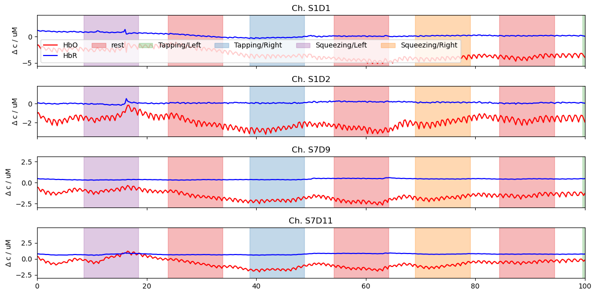
Plotting Time Series Using Matplotlib
Preprocess and select the data for visualization. Afterwards use standard matplotlib functions to create line plots.
The function cedalion.vis.blocks.plot_stim_markers highlights stimulation periods.
[5]:
import cedalion.vis.blocks as vbx

# calculate HbO/HbR from raw data
dpf = xr.DataArray(
        [6, 6],
        dims="wavelength",
        coords={"wavelength": rec["amp"].wavelength},
    )
rec["conc"] = cedalion.nirs.cw.beer_lambert(
    rec["amp"], rec.geo3d, dpf, spectrum="prahl"
)
# rename events
rec.stim.cd.rename_events(
        {"1": "rest", "2": "Tapping/Left", "3": "Tapping/Right", "4": "Squeezing/Left", "5": "Squeezing/Right"}
    )

# select which time series we work with
ts = rec["conc"]

# Thanks to the xarray DataArray structure, we can easily select the data we want to plot
# plot four channels and their stim markers
f, ax = plt.subplots(4, 1, sharex=True, figsize=(12, 6))
for i, ch in enumerate(["S1D1", "S1D2", "S7D9", "S7D11"]):
    ax[i].plot(ts.time, ts.sel(channel=ch, chromo="HbO"), "r-", label="HbO")
    ax[i].plot(ts.time, ts.sel(channel=ch, chromo="HbR"), "b-", label="HbR")
    ax[i].set_title(f"Ch. {ch}")

    # add stim markers using Cedalion's plot_stim_markers function
    vbx.plot_stim_markers(ax[i], rec.stim, y=1)
    ax[i].set_ylabel(r"$\Delta$ c / uM")

ax[0].legend(ncol=6)
ax[3].set_label("time / s")
ax[3].set_xlim(0,100)
plt.tight_layout()
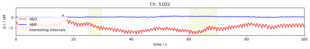
The function cedalion.vis.blocks.plot_segments can be used to highlight time intervals
[6]:
import cedalion.vis.blocks as vbx

f, ax = plt.subplots(1, 1, sharex=True, figsize=(12, 2))
ch = "S1D2"
ax.plot(ts.time, ts.sel(channel=ch, chromo="HbO"), "r-", label="HbO")
ax.plot(ts.time, ts.sel(channel=ch, chromo="HbR"), "b-", label="HbR")
ax.set_title(f"Ch. {ch}")

segments = [(25,30), (60,70)]

vbx.plot_segments(ax, segments, fmt={"facecolor": "y", "alpha": 0.1}, label="interesting intervals")

ax.legend(loc="lower left")
ax.set_ylabel(r"$\Delta$ c / uM")
ax.set_xlabel("time / s")
ax.set_xlim(0,100)
plt.tight_layout()
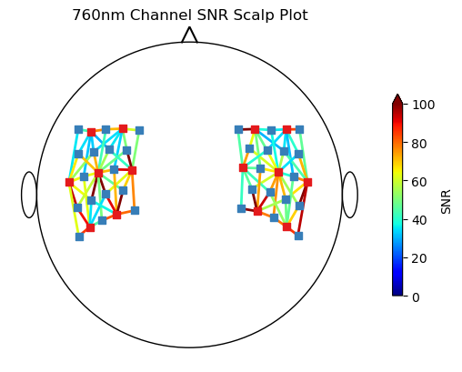
Scalp Plot
Plots a metric, e.g. channel quality or amplitude at a time point on the scalp.
[7]:
from cedalion.vis.anatomy import scalp_plot

n_channels = len(rec["amp"].channel)
# Calculate channel SNR to display as a metric in the plot
snr, snr_mask = cedalion.sigproc.quality.snr(rec["amp"], 3)
# the plots "metric" input needs dimension (nchannels,)
# so we focus on the 760nm wavelength for each channel
snr_metric = snr.sel(wavelength="760")

# Create scalp plot showing SNR in each channel
fig, ax = plt.subplots(1, 1)

scalp_plot(
    rec["amp"],
    rec.geo3d,
    snr_metric,
    ax,
    cmap="jet",
    title="760nm Channel SNR Scalp Plot",
    vmin=0,
    vmax=n_channels,
    cb_label="SNR",
)
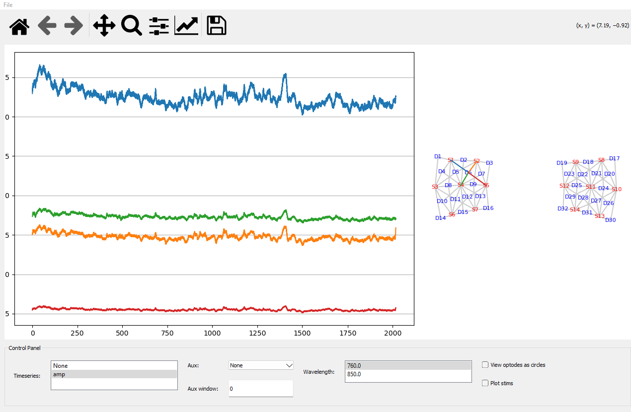
Plotting Time Series Using an interactive GUI
run_vis() from the vis.timeseries package
[8]:
from cedalion.vis.misc import time_series_gui

# this calls a GUI to interactively select channels from a 2D probe.
# Input is a recording container, you can choose which time series (e.g. raw, OD, concentrations) in the container  to plot

# UNCOMMENT to use the GUI. Commented out for documentation autogeneration purposes.
#time_series_gui.run_vis(rec)
Plotting an fNIRS Montage in 3D
The function cedalion.vis.anatomy.plot_montage3D() gives a quick overview of optode and landmark positions.
[9]:
from cedalion.vis.anatomy import plot_montage3D

# use the plot_montage3D() function. It requires a recording container and a geo3d object
plot_montage3D(rec["amp"], rec.geo3d)
Visualization Building Blocks
The subpackage cedalion.vis.blocks contains wrappers around matplotlib and pyvista functionality that allow to assemble larger visualizations. In the following these will be used to build 3D plots of the scalp and brain.
Currently the following functions are available:
[10]:
import cedalion.vis.blocks as vbx

for name in vbx.__all__:
    print(name)
plot_stim_markers
plot_segments
plot_surface
plot_labeled_points
plot_vector_field
camera_at_cog
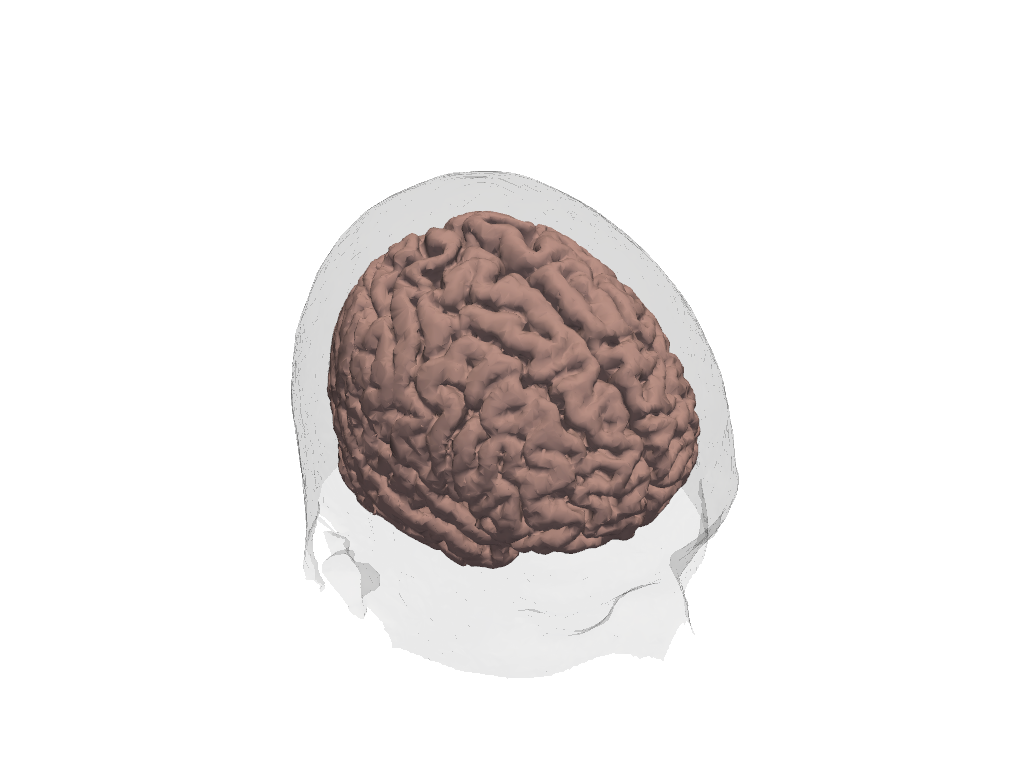
Plotting Headmodels
Scalp and brain tissue are represented by surfaces. Plot theses surfaces for the loaded Colin27 headmodel by using plot_surface().
To point the camera at the center of gravity of a surface use camera_at_cog().
[11]:
import cedalion.vis.blocks as vbx

plt = pv.Plotter()
vbx.plot_surface(plt, head.brain, color="#d3a6a1")
vbx.plot_surface(plt, head.scalp, opacity=.1)

vbx.camera_at_cog(plt, head.scalp, (-300,300,300), fit_scene=False)
plt.show()
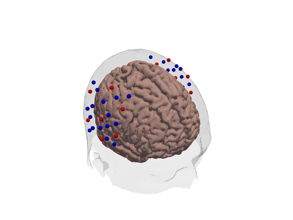
Adding a montage to the headmodel
For this the montage has to be registered to the headmodel’s scalp first. Then we use plot_labeled_points
[12]:
import cedalion.vis.blocks as vbx

geo3d_snapped = head.align_and_snap_to_scalp(rec.geo3d)

# now we plot the head same as before...
plt = pv.Plotter()
vbx.plot_surface(plt, head.brain, color="#d3a6a1")
vbx.plot_surface(plt, head.scalp, opacity=.1)
# but use the plot_labeled_points() function to add the snapped geo3d.
# The flag "show_labels" can be used to show the source, detector, and landmark names
vbx.plot_labeled_points(plt, geo3d_snapped, show_labels=False)
plt.show()
We can also easily remove the EEG landmarks for a better visual…
[13]:
import cedalion.vis.blocks as vbx

# keep only points that are not of type "landmark", i.e. source and detector points
geo3d_snapped = geo3d_snapped[geo3d_snapped.type != cdc.PointType.LANDMARK]

# now we plot the head same as before...
plt = pv.Plotter()
vbx.plot_surface(plt, head.brain, color="#d3a6a1")
vbx.plot_surface(plt, head.scalp, opacity=.1)
# but use the plot_labeled_points() function to add the snapped geo3d.
# The flag "show_labels" can be used to show the source, detector, and landmark names
vbx.plot_labeled_points(plt, geo3d_snapped, show_labels=True)
plt.show()
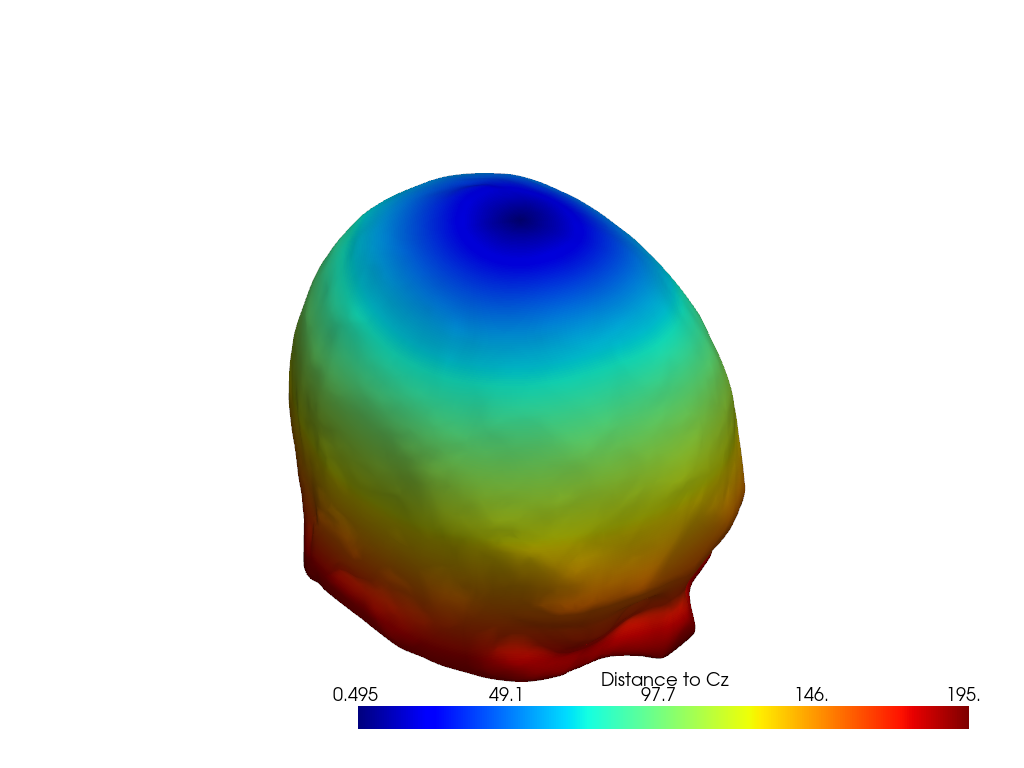
To plot a metric on a surface, pass an array to the color param.
Extra keywords (like cmap or scalar_bar_args in this example) are passed-through to pyvista.
[14]:
import cedalion.vis.blocks as vbx

plt = pv.Plotter()

dist_to_cz = xrutils.norm(head.scalp.vertices - head.landmarks.loc["Cz"], dim=head.crs)

vbx.plot_surface(
    plt,
    head.scalp,
    color=dist_to_cz,
    cmap="jet",
    scalar_bar_args={"title": "Distance to Cz"},
)

plt.show()
To plot a metric on the brain surface and to include the result in a matplotlib figure, use cedalion.vis.anatomy.plot_brain_in_axes
[15]:
from cedalion.vis.anatomy import plot_brain_in_axes

f, ax = p.subplots(1,2, figsize=(10,5))

dist_to_nz = xrutils.norm(head.brain.vertices - head.landmarks.loc["Nz"], dim=head.crs)

for i, cam_pos in enumerate([[-450,0,0], [100,100,600]]):
    plot_brain_in_axes(
        rec["amp"],
        geo3d_snapped,
        dist_to_nz,
        head.brain,
        ax[i],
        title="Distance to Cz",
        vmin=None,
        vmax=None,
        cmap="inferno",
        cb_label="distance",
        camera_pos=cam_pos,
    )
p.tight_layout()
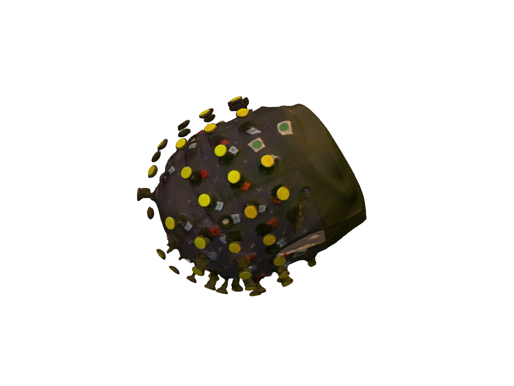
Surface Plot of 3D Scans
Uses the same function as for head models, plot_surface()
[16]:
import cedalion.vis.blocks as vbx

plt = pv.Plotter()
vbx.plot_surface(plt, pscan, opacity=1.0)
vbx.camera_at_cog(plt, pscan, [-250,  -150, -340], up=(1,-1,0), fit_scene=True)
plt.show()
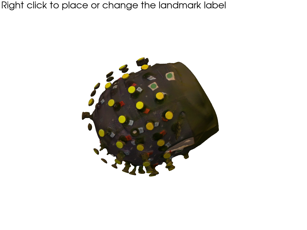
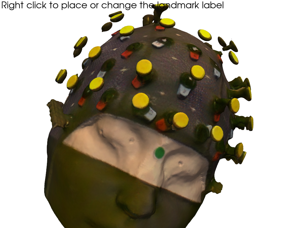
Interactive 3D Plot to select Landmarks
using plot_surface with pick_landmarks = ['Nz', 'Iz', 'Cz', 'Lpa', 'Rpa']. Here we use a photogrammetric scan, and the landmarks are indicated by green dots. Right-clicking again on an existing landmark changes the label.
[17]:
import cedalion.vis.blocks as vbx

plt = pv.Plotter()
vbx.camera_at_cog(plt, pscan, [-250,  -150, -340], up=(1,-1,0), fit_scene=True)
get_landmarks = vbx.plot_surface(plt, pscan, opacity=1.0, pick_landmarks = ['Nz', 'Iz', 'Cz', 'Lpa', 'Rpa'])
plt.show(interactive = True)
[18]:
# for documentation purposes and to enable automatically rendered example notebooks we provide the hand-picked coordinates here too.
landmark_labels = ['Nz', 'Iz', 'Cz', 'Lpa', 'Rpa']
landmark_coordinates = [np.array([14.00420712, -7.84856869, 449.77840004]),
                                  np.array([99.09920059, 29.72154755, 620.73876117]),
                                  np.array([161.63815139, -48.49738938, 494.91210993]),
                                  np.array([82.8771277, 79.79500128, 498.3338802]),
                                  np.array([15.17214095, -60.56186128, 563.29621021])]

# Uncomment the following lines if you want to see your own picked results. When you are done, run' get_landmarks() ' to retrieve the landmarks.
#landmarks = get_landmarks()
#landmark_labels = landmarks.label.values
#landmark_coordinates = landmarks.values
display(landmark_labels)
['Nz', 'Iz', 'Cz', 'Lpa', 'Rpa']
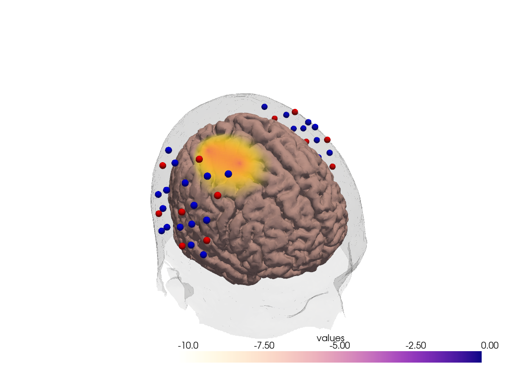
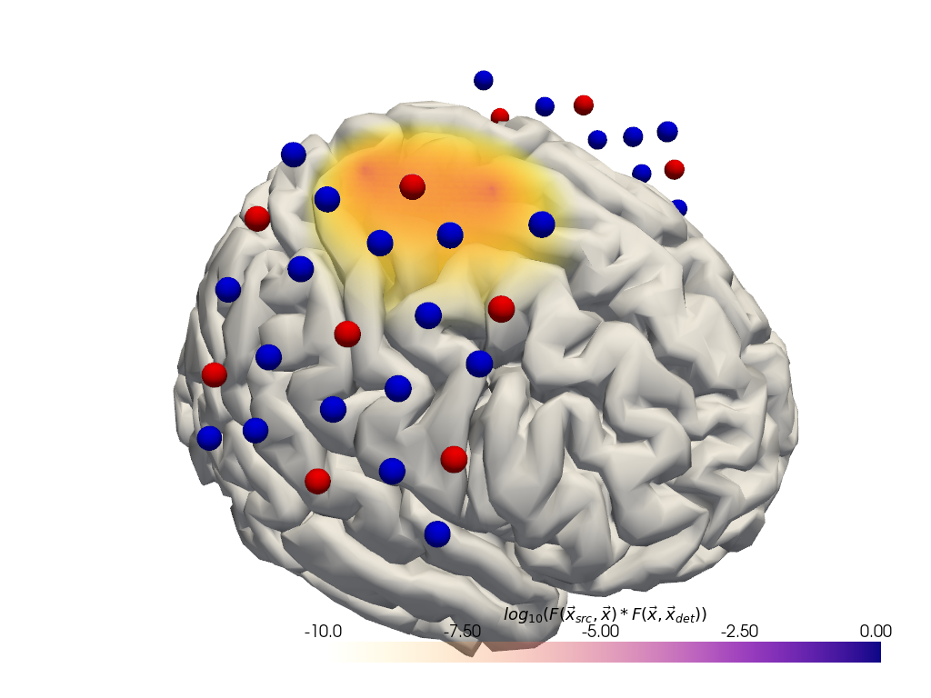
Plot Probe Fluence / Sensitivity on Cortex
Plot the fluence between a source-detector pair, or the accumulated sensitivity profile on the cortex
Fluence between two optodes
[19]:
import cedalion.vis.blocks as vbx

# pull fluence values from the corresponding source and detector pair

with FluenceFile(fluence_fname) as fluence_file:
    f = fluence_file.get_fluence("S12", 760) * fluence_file.get_fluence("D19", 760)

f = np.log10(np.clip(f, min=f[f > 0].min()))
vf = pv.wrap(f)

plt = pv.Plotter()

plt.add_volume(
    vf,
    log_scale=False,
    cmap="plasma_r",
    clim=(-10, -0),
    scalar_bar_args={
        "title": r"$log_{10}("
        r"F(\vec{x}_{src},\vec{x}) * F(\vec{x}, \vec{x}_{det})"
        ")$"
    },
)
vbx.plot_surface(plt, head.brain, color="w")
vbx.plot_labeled_points(plt, geo3d_snapped, show_labels=False)
vbx.camera_at_cog(plt, head.brain, rpos=[300, 150, 150])
plt.show()
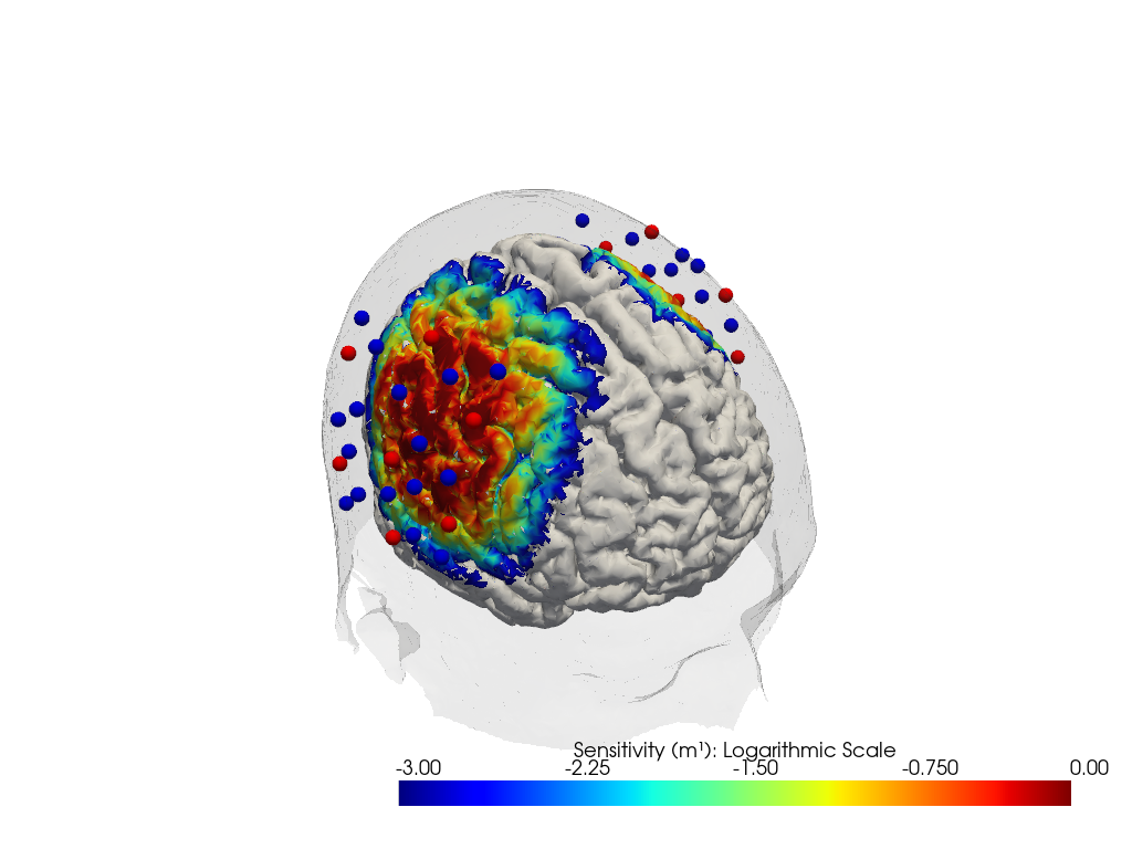
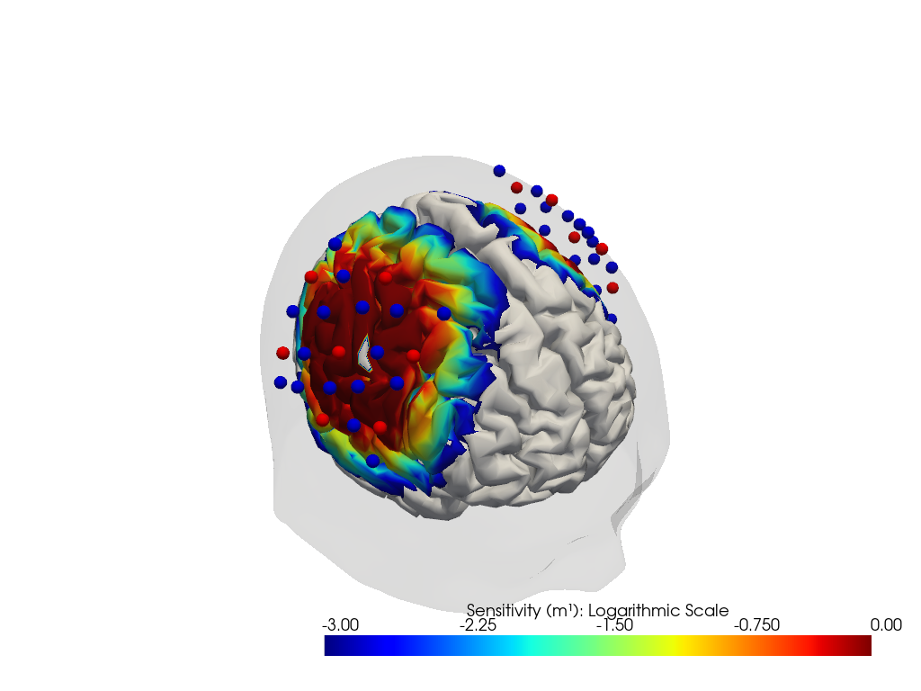
Plot Sensitivity Profile on Cortex
Using the calculated fluence. This will be simplified in the future to make it easier for you.
[20]:
import cedalion.vis.anatomy.sensitivity_matrix as sensitivity_matrix

plotter = sensitivity_matrix.Main(
    sensitivity=Adot,
    brain_surface=head.brain,
    head_surface=head.scalp,
    labeled_points=geo3d_snapped,
)
plotter.plot(high_th=0, low_th=-3)
plotter.plt.show()
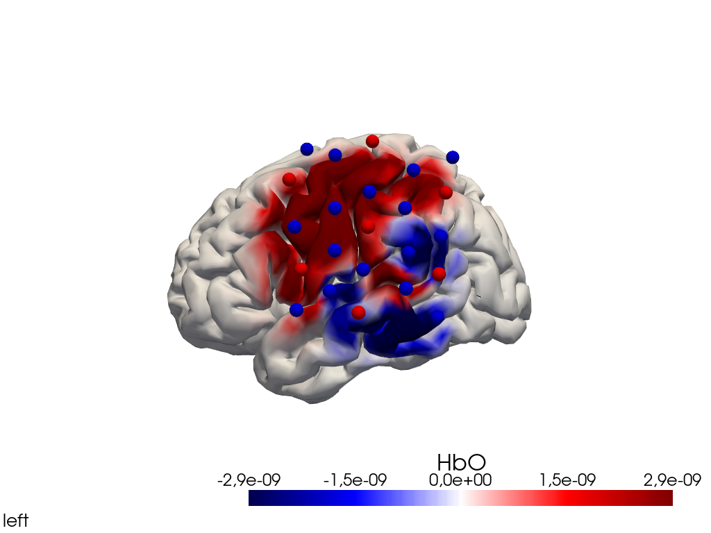
Plot ImageRecon HRF Activation (from HD fNIRS/DOT) on Cortex or Scalp
Since this requires a lot of preprocessing, please use the Image Reconstruction Jupyter Example Notebook HERE. There you will be able to generate the following types of plots yourself. Here, we load saved examples generated with the corresponding function calls:
[21]:
from cedalion.vis.anatomy import scalp_plot_gif

# plot activity in channels on a scalp map over time

""" scalp_plot_gif(
        data_ts,
        geo3d,
        filename = filename_scalp,
        time_range=(-5,30,0.5)*units.s,
        scl=(-0.01, 0.01),
        fps=6,
        optode_size=6,
        optode_labels=True,
        str_title='850 nm'
    ) """
[21]:
" scalp_plot_gif( \n data_ts, \n geo3d, \n filename = filename_scalp, \n time_range=(-5,30,0.5)*units.s,\n scl=(-0.01, 0.01), \n fps=6, \n optode_size=6, \n optode_labels=True, \n str_title='850 nm' \n ) "
[22]:
from cedalion.vis.anatomy import image_recon_view

# plot reconstructed  activity (here HbO) in a 3D view over time on the brain surface

""" image_recon_view(
        X_ts,  # time series data; can be 2D (static) or 3D (dynamic)
        head,
        cmap='seismic',
        clim=clim,
        view_type='hbo_brain',
        view_position='left',
        title_str='HbO',
        filename=filename_view,
        SAVE=True,
        time_range=(-5,30,0.5)*units.s,
        fps=6,
        geo3d_plot = geo3d_plot,
        wdw_size = (1024, 768)
) """
[22]:
" image_recon_view(\n X_ts, # time series data; can be 2D (static) or 3D (dynamic)\n head,\n cmap='seismic',\n clim=clim,\n view_type='hbo_brain',\n view_position='left',\n title_str='HbO',\n filename=filename_view,\n SAVE=True,\n time_range=(-5,30,0.5)*units.s,\n fps=6,\n geo3d_plot = geo3d_plot,\n wdw_size = (1024, 768)\n) "
[23]:
from cedalion.vis.anatomy import image_recon_view
# plot reconstructed  activity (here HbO) in a 3D view at any single
# time point on the brain surface

"""
    # selects the nearest time sample at t=10s in X_ts
    X_ts = X_ts.sel(time=10*units.s, method="nearest")

    image_recon_view(
        X_ts,  # time series data; can be 2D (static) or 3D (dynamic)
        head,
        cmap='seismic',
        clim=clim,
        view_type='hbo_brain',
        view_position='left',
        title_str='HbO',
        filename=filename_view,
        SAVE=True,
        time_range=(-5,30,0.5)*units.s,
        fps=6,
        geo3d_plot = geo3d_plot,
        wdw_size = (1024, 768)
) """
[23]:
' \n # selects the nearest time sample at t=10s in X_ts\n X_ts = X_ts.sel(time=10*units.s, method="nearest")\n\n image_recon_view(\n X_ts, # time series data; can be 2D (static) or 3D (dynamic)\n head,\n cmap=\'seismic\',\n clim=clim,\n view_type=\'hbo_brain\',\n view_position=\'left\',\n title_str=\'HbO\',\n filename=filename_view,\n SAVE=True,\n time_range=(-5,30,0.5)*units.s,\n fps=6,\n geo3d_plot = geo3d_plot,\n wdw_size = (1024, 768)\n) '
[24]:
from cedalion.vis.anatomy import image_recon_multi_view

# plot reconstructed activity (here HbO) in from all 3D views over time on the brain surface

""" image_recon_multi_view(
        X_ts,  # time series data; can be 2D (static) or 3D (dynamic)
        head,
        cmap='seismic',
        clim=clim,
        view_type='hbo_brain',
        title_str='HbO',
        filename=filename_multiview,
        SAVE=True,
        time_range=(-5,30,0.5)*units.s,
        fps=6,
        geo3d_plot = None #  geo3d_plot,
        wdw_size = (1024, 768)
) """
[24]:
" image_recon_multi_view(\n X_ts, # time series data; can be 2D (static) or 3D (dynamic)\n head,\n cmap='seismic',\n clim=clim,\n view_type='hbo_brain',\n title_str='HbO',\n filename=filename_multiview,\n SAVE=True,\n time_range=(-5,30,0.5)*units.s,\n fps=6,\n geo3d_plot = None # geo3d_plot,\n wdw_size = (1024, 768)\n) "
[25]:
from cedalion.vis.anatomy import image_recon_multi_view
# plot reconstructed activity (here HbO) in from all 3D views over time on the scalp surface

""" image_recon_multi_view(
        X_ts,  # time series data; can be 2D (static) or 3D (dynamic)
        head,
        cmap='seismic',
        clim=clim,
        view_type='hbo_scalp',
        title_str='HbO',
        filename=filename_multiview,
        SAVE=True,
        time_range=(-5,30,0.5)*units.s,
        fps=6,
        geo3d_plot = geo3d_plot,
        wdw_size = (1024, 768)
) """
[25]:
" image_recon_multi_view(\n X_ts, # time series data; can be 2D (static) or 3D (dynamic)\n head,\n cmap='seismic',\n clim=clim,\n view_type='hbo_scalp',\n title_str='HbO',\n filename=filename_multiview,\n SAVE=True,\n time_range=(-5,30,0.5)*units.s,\n fps=6,\n geo3d_plot = geo3d_plot,\n wdw_size = (1024, 768)\n) "
Colors
The subpackage cedalion.vis.colors provides color and colormap definitions.
A colormap for p-values:
[26]:
from cedalion.vis.colors import p_values_cmap

norm, cmap = p_values_cmap()
display(cmap)

[27]:
from cedalion.vis.colors import threshold_cmap

norm, cmap = threshold_cmap("sci_cmap_gt", 0,1,0.75, higher_is_better=True)
display(cmap)
norm, cmap = threshold_cmap("sci_cmap_lt", 0,1,0.75, higher_is_better=False)
display(cmap)


[28]:
from cedalion.vis.colors import mask_cmap

norm, cmap = mask_cmap(true_is_good=True)
display(cmap)
norm, cmap = mask_cmap(true_is_good=False)
display(cmap)


References
[29]:
cedalion.bib.dump_to_notebook()
Methods used
| [1] | Tucker2022 | cedalion.io.snirf.read_snirf | Stephen Tucker, Jay Dubb, Sreekanth Kura, Alexander von Lühmann, Robert Franke, Jörn M. Horschig, Samuel Powell, Robert Oostenveld, Michael Lührs, Édouard Delaire, Zahra M. Aghajan, Hanseok Yun, Meryem A. Yücel, Qianqian Fang, Theodore J. Huppert, Blaise deB. Frederick, Luca Pollonini, David A. Boas, and Robert Luke. Introduction to the shared near infrared spectroscopy format. Neurophotonics, 10(1):013507, 2022. doi:10.1117/1.NPh.10.1.013507. |
| [2] | Fang2009 | cedalion.data.get_precomputed_fluence, cedalion.data.get_precomputed_sensitivity | Qianqian Fang and David A Boas. Monte carlo simulation of photon migration in 3d turbid media accelerated by graphics processing units. Optics express, 17(22):20178–20190, 2009. doi:10.1364/OE.17.020178. |
| [3] | Yu2018 | cedalion.data.get_precomputed_fluence, cedalion.data.get_precomputed_sensitivity | Leiming Yu, Fanny Nina-Paravecino, David Kaeli, and Qianqian Fang. Scalable and massively parallel monte carlo photon transport simulations for heterogeneous computing platforms. Journal of biomedical optics, 23(1):010504–010504, 2018. doi:10.1117/1.JBO.23.1.010504. |
| [4] | Yan2020 | cedalion.data.get_precomputed_fluence, cedalion.data.get_precomputed_sensitivity | Shijie Yan and Qianqian Fang. Hybrid mesh and voxel based monte carlo algorithm for accurate and efficient photon transport modeling in complex bio-tissues. Biomedical Optics Express, 11(11):6262–6270, 2020. doi:10.1364/BOE.409468. |
| [5] | Holmes1998 | cedalion.data.get_colin27_headmodel_files | Colin J. Holmes, Rick Hoge, Louis Collins, Roger Woods, Arthur W. Toga, and Alan C. Evans. Enhancement of mr images using registration for signal averaging. Journal of Computer Assisted Tomography, 22(2):324–333, March 1998. doi:10.1097/00004728-199803000-00032. |
| [6] | Fischl2012 | cedalion.data.get_colin27_headmodel_files | Bruce Fischl. FreeSurfer. NeuroImage, 62(2):774–781, 2012. doi:10.1016/j.neuroimage.2012.01.021. |
| [7] | Schaefer2018 | cedalion.data.get_colin27_headmodel_files | Alexander Schaefer, Ru Kong, Evan M Gordon, Timothy O Laumann, Xi-Nian Zuo, Avram J Holmes, Simon B Eickhoff, and BT Thomas Yeo. Local-global parcellation of the human cerebral cortex from intrinsic functional connectivity mri. Cerebral cortex, 28(9):3095–3114, 2018. doi:10.1093/cercor/bhx179. |
| [8] | Delpy1988 | cedalion.nirs.cw.beer_lambert, cedalion.nirs.cw.int2od, cedalion.nirs.cw.od2conc | D. T. Delpy, M. Cope, P. van der Zee, S. Arridge, S. Wray, and J. Wyatt. Estimation of optical pathlength through tissue from direct time of flight measurement. Physics in Medicine and Biology, 33(12):1433–1442, 1988. doi:10.1088/0031-9155/33/12/008. |
| [9] | Villringer1997 | cedalion.nirs.cw.beer_lambert, cedalion.nirs.cw.int2od, cedalion.nirs.cw.od2conc | Arno Villringer and Britton Chance. Non-invasive optical spectroscopy and imaging of human brain function. Trends in Neurosciences, 20(10):435–442, 1997. doi:10.1016/S0166-2236(97)01132-6. |
| [10] | Prahl1998 | cedalion.nirs.common.get_extinction_coefficients | Scott A. Prahl. Optical absorption of hemoglobin. Oregon Medical Laser Center, online resource, 1998. URL: https://omlc.org/spectra/hemoglobin/. |
| [11] | Huppert2009 | cedalion.sigproc.quality.snr | Theodore J. Huppert, Solomon G. Diamond, Maria A. Franceschini, and David A. Boas. Homer: a review of time-series analysis methods for near-infrared spectroscopy of the brain. Appl. Opt., 48(10):D280–D298, Apr 2009. doi:https://doi.org/10.1364/AO.48.00D280. |