Using Channel Variance as Proxy for Measurement Noise and as a Weight for Global Physiology Removal
To improve statistics, channel pruning might not always be the way. An alternative is to use channel weights in the calculation of averages (e.g. across subjects) or image reconstruction. One way of weighting channels is by their estimated measurement noise. Variance can be a proxy of measurement noise, e.g. when calculated across trials of the same condition (within subject) or across time on the residual after GLM fit. This notebook is WIP to provide help to explore this approach with a helper function (quality.measurement_variance) for this purpose. We will first create an intuition how to use the quality.measurement_variance function, and then use the output for weighted global physiology removal with physio.global_physio_subtract.
[1]:
# This cells setups the environment when executed in Google Colab.
try:
    import google.colab
    !curl -s https://raw.githubusercontent.com/ibs-lab/cedalion/dev/scripts/colab_setup.py -o colab_setup.py
    # Select branch with --branch "branch name" (default is "dev")
    %run colab_setup.py
except ImportError:
    pass
[2]:
import matplotlib.pyplot as plt
from matplotlib.colors import LinearSegmentedColormap
import numpy as np

import cedalion
import cedalion.data as datasets
import cedalion.nirs
import cedalion.sigproc.quality as quality
import cedalion.sigproc.motion as motion
from cedalion import units
import cedalion.xrutils as xrutils
[3]:
# some plotting helper functions for this notebook

import xarray as xr

def plot_heatmap(da, cov_wavelength=None, figsize=(12, 4), cmap=None):
    dims = da.dims

    # VARIANCE CASE: dims = ("channel", "wavelength")
    if set(dims) == {"channel", "wavelength"}:
        # Convert to pandas DataFrame so that rows = channels, cols = wavelengths
        df = da.to_pandas()

        # We want channels on the x-axis, wavelengths on the y-axis.
        #   df.values has shape (n_channels, n_wavelengths), so transpose → (n_wavelengths, n_channels)
        arr = df.values.T

        x_labels = df.index.tolist()         # channel names
        y_labels = [str(int(wl)) for wl in df.columns]  # wavelength values as strings

        x_dim_name = "channel"
        y_dim_name = "wavelength"
        cbar_label = "Variance"

    # COVARIANCE CASE: dims = ("wavelength", "channel1", "channel2")
    elif set(dims) == {"wavelength", "channel1", "channel2"}:
        if cov_wavelength is None:
            raise ValueError(
                "When da.dims == ('wavelength','channel1','channel2'), you must supply cov_wavelength."
            )
        # Extract the 2D slice at that wavelength
        da2d = da.sel(wavelength=cov_wavelength)
        # Make sure dims are in order (channel1, channel2)
        da2d = da2d.transpose("channel1", "channel2")

        arr = da2d.values  # shape = (n_channel1, n_channel2)

        x_labels = da2d.coords["channel2"].values.tolist()
        y_labels = da2d.coords["channel1"].values.tolist()

        x_dim_name = "channel2"
        y_dim_name = "channel1"
        cbar_label = f"Covariance (λ={cov_wavelength})"

    else:
        raise ValueError(f"Unsupported DataArray dimensions: {dims}")

    # Plot the 2D array with imshow
    fig, ax = plt.subplots(figsize=figsize)
    im = ax.imshow(arr, aspect="auto", cmap=cmap)

    # Set x-axis ticks/labels
    ax.set_xticks(range(len(x_labels)))
    ax.set_xticklabels(x_labels, rotation=90, fontsize=8)

    # Set y-axis ticks/labels
    ax.set_yticks(range(len(y_labels)))
    ax.set_yticklabels(y_labels, fontsize=8)

    # Label axes from the dimension names
    ax.set_xlabel(x_dim_name)
    ax.set_ylabel(y_dim_name)

    # Add a colorbar
    cbar = fig.colorbar(im, ax=ax)
    cbar.set_label(cbar_label)

    plt.tight_layout()
    return fig, ax


def plot_selected_channels(
    rec: xr.Dataset,
    channels: list,
    wavelength: float,
    da_name: str = "od",
    figsize: tuple = (12, 4),
    time_xlim: tuple = (0, 500)
):

    fig, ax = plt.subplots(1, 1, figsize=figsize)

    for ch in channels:
        series = rec[da_name].sel({ "channel": ch, "wavelength": wavelength })
        ax.plot(rec[da_name].time, series, label=f"{ch} {wavelength}nm")

    ax.legend()
    ax.set_xlim(*time_xlim)
    ax.set_xlabel("time / s")
    ax.set_ylabel("Signal intensity / a.u.")
    plt.show()
Channel Variance as a Proxy for Measurement Noise
Plain Channel Variance
Note: channel variance can only be a proxy for measurement noise if calculated OD or CONC. Do not calculate on raw intensity.
[4]:
# get example finger tapping dataset
rec = datasets.get_fingertapping()
rec["od"] = cedalion.nirs.cw.int2od(rec["amp"])
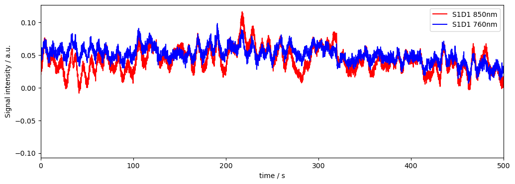
# Plot some data for visual validation
f,ax = plt.subplots(1,1, figsize=(12,4))
ax.plot( rec["od"].time, rec["od"].sel(channel="S1D1", wavelength="850"), "r-", label="S1D1 850nm")
ax.plot( rec["od"].time, rec["od"].sel(channel="S1D1", wavelength="760"), "b-", label="S1D1 760nm")
plt.legend()
ax.set_xlim(0, 500)
ax.set_xlabel("time / s")
ax.set_ylabel("Signal intensity / a.u.")
[4]:
Text(0, 0.5, 'Signal intensity / a.u.')
Calculate variance of all channels and display results
[5]:
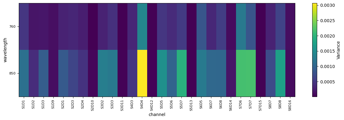
# calculate variance of optical density (OD) measurements for all channels and wavelengths
od_var = quality.measurement_variance(rec["od"])

fig, ax = plot_heatmap(od_var)
plt.show()
/home/runner/miniconda3/envs/cedalion/lib/python3.11/site-packages/xarray/core/variable.py:315: UnitStrippedWarning: The unit of the quantity is stripped when downcasting to ndarray.
  data = np.asarray(data)
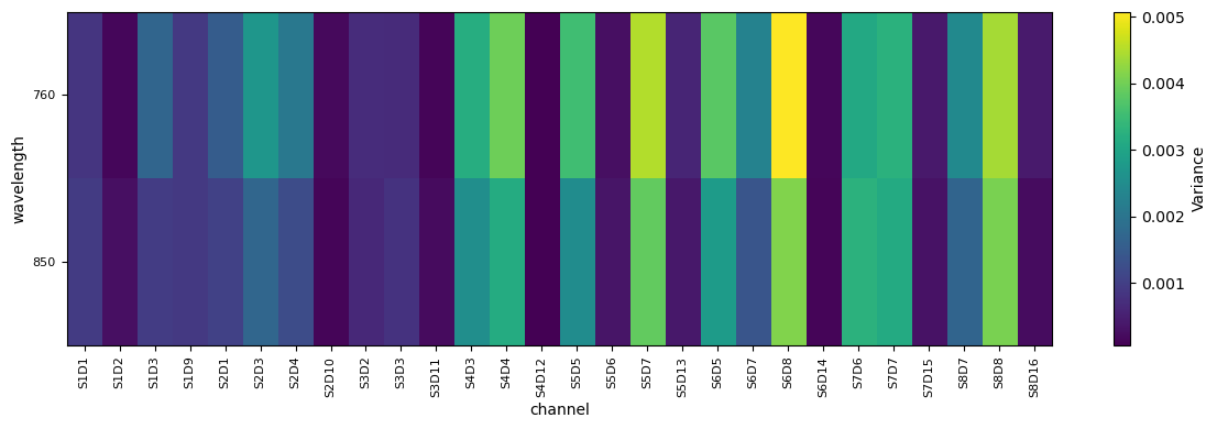
From the plot above we can identify S6D8 (760nm) as a channel with high variance and and S1D2 (760nm) as a channel with low variance. S7D6 is somewhere inbetween. Lets investigate how the corresponding time series looks like.
[6]:
# Plot some data for visual validation
f,ax = plt.subplots(1,1, figsize=(12,4))
ax.plot( rec["od"].time, rec["od"].sel(channel="S6D8", wavelength="760"), "r-", label="S6D8 760nm")
ax.plot( rec["od"].time, rec["od"].sel(channel="S1D2", wavelength="760"), "b-", label="S1D2 760nm")
ax.plot( rec["od"].time, rec["od"].sel(channel="S7D6", wavelength="760"), "y-", label="S7D6 760nm")
plt.legend()
ax.set_xlim(0, 500)
ax.set_xlabel("time / s")
ax.set_ylabel("Signal intensity / a.u.")
[6]:
Text(0, 0.5, 'Signal intensity / a.u.')
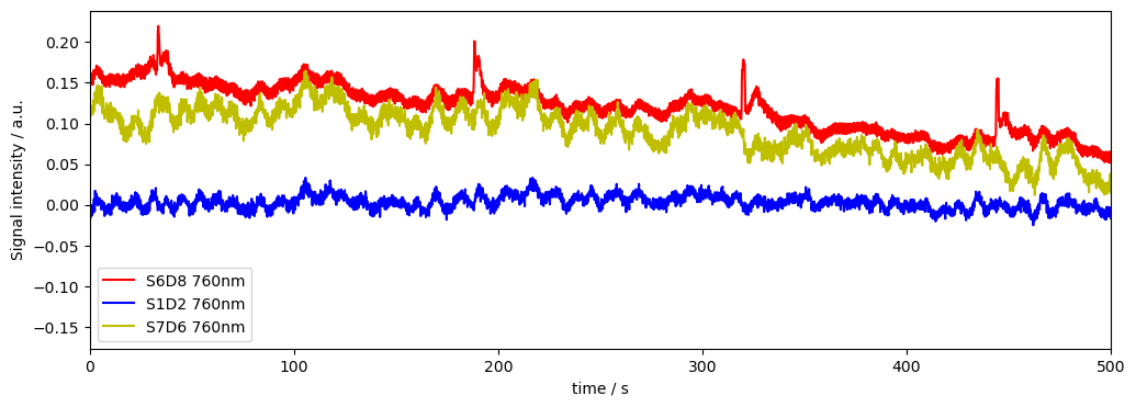
We can see that the Channel with high variance has motion artifacts. These can be removed with motion correction methods and we can recalculate the variance to see if this helped. If we don’t, and use the channel variance as is for weighting in further processing, the channel with motion artifacts will be downweighted, as it has higher variance.
[7]:
# motion correction using the wavelet and tddr methods
rec["od_corrected"] = motion.tddr(rec["od"])
rec["od_corrected"] = motion.wavelet(rec["od_corrected"])


# Plot corrected data for visual validation
f,ax = plt.subplots(1,1, figsize=(12,4))
ax.plot( rec["od_corrected"].time, rec["od_corrected"].sel(channel="S6D8", wavelength="760"), "r-", label="S6D8 760nm")
ax.plot( rec["od_corrected"].time, rec["od_corrected"].sel(channel="S1D2", wavelength="760"), "b-", label="S1D2 760nm")
ax.plot( rec["od_corrected"].time, rec["od_corrected"].sel(channel="S7D6", wavelength="760"), "y-", label="S7D6 760nm")
plt.legend()
ax.set_xlim(0, 500)
ax.set_xlabel("time / s")
ax.set_ylabel("Signal intensity / a.u.")

# calculate variance on the corrected signal
od_var2 = quality.measurement_variance(rec["od_corrected"])


## Display results as a heatmap
fig, ax = plot_heatmap(od_var2)
plt.show()
/home/runner/miniconda3/envs/cedalion/lib/python3.11/site-packages/xarray/core/variable.py:315: UnitStrippedWarning: The unit of the quantity is stripped when downcasting to ndarray.
  data = np.asarray(data)
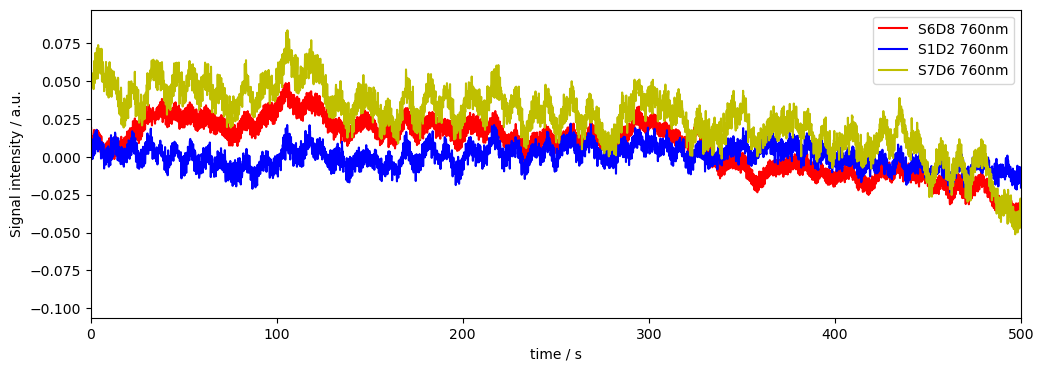
We can see that motion correction took care of some variance (and therefore fixed some channels like S6D8), but not all of it, S4D4 remains partially noisy.
Channel variance under consideration of flagged bad channels
There are cases in which we don’t trust channel variance as a proxy for measurement noise. Examples are saturated channels. We could also want to penalize channels with motion artifacts particulalry strongly and for instance kick out S4D4, which did only partially profit from artifact rejection. For this we can provide a list of “bad” channels and a custom weight.
[8]:
# lets assume we do not want to do motion correction and channel S1D1 is saturated.
# We give S1D1 it a constant value of 1V with only the measurement noise of the system of 10mV
rec["amp"].loc[{"channel": "S1D1"}] = (1 + np.random.normal(0, 10e-3, rec["amp"].sel(channel="S1D1").shape))*units.V

# now convert the signal to optical density
rec["od"] = cedalion.nirs.cw.int2od(rec["amp"])


# Plot some data for visual validation
f,ax = plt.subplots(1,1, figsize=(12,4))
ax.plot( rec["od"].time, rec["od"].sel(channel="S1D1", wavelength="760"), "b-", label="S1D1 760nm")
ax.plot( rec["od"].time, rec["od"].sel(channel="S4D4", wavelength="850"), "r-", label="S4D4 850nm")
plt.legend()
ax.set_xlim(0, 500)
ax.set_xlabel("time / s")
ax.set_ylabel("Signal intensity / a.u.")
[8]:
Text(0, 0.5, 'Signal intensity / a.u.')
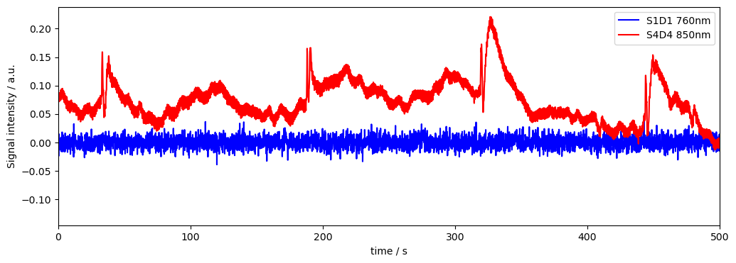
Looking at the resulting variance of the saturated channel S1D2 and comparing it with the noisy (motion artifact) channel S4D4…
[9]:
# calculate variance of optical density (OD) measurements for all channels and chromophores
od_var = quality.measurement_variance(rec["od"])

# print channel S1D1 760nm and channel S6D8 760nm variance
print("S1D1 760nm variance:", od_var.sel(channel="S1D1", wavelength="760").values)
print("S4D4 760nm variance:", od_var.sel(channel="S4D4", wavelength="850").values)
S1D1 760nm variance: 9.990592569306349e-05
S4D4 760nm variance: 0.0031518609824904144
/home/runner/miniconda3/envs/cedalion/lib/python3.11/site-packages/xarray/core/variable.py:315: UnitStrippedWarning: The unit of the quantity is stripped when downcasting to ndarray.
  data = np.asarray(data)
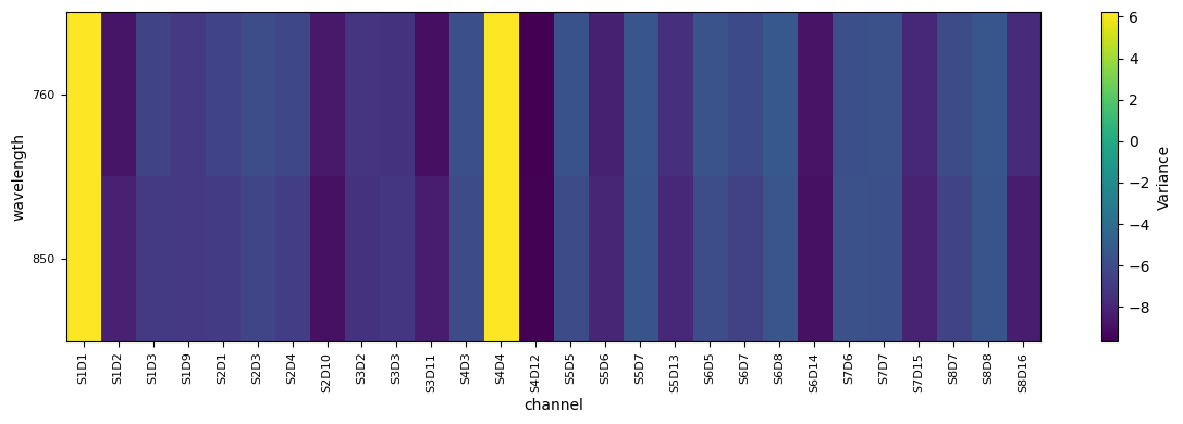
we can tell that the metric cannot account for saturation, and we should manually drop / downweight the saturated channel.
[10]:
list_bad_channels = ["S1D1", "S4D4"]
bad_rel_var = 1e5 # we use a large factor that will be multiplied with the channel variance to effectively remove the channel from the analysis wherever it is weighted by its variance

od_var = quality.measurement_variance(rec["od"], list_bad_channels, bad_rel_var)

## Display results as a heatmap, this time on a logarithmic scale as the penalty factor is large
fig, ax = plot_heatmap(np.log(od_var))
plt.show()
/home/runner/miniconda3/envs/cedalion/lib/python3.11/site-packages/xarray/core/variable.py:315: UnitStrippedWarning: The unit of the quantity is stripped when downcasting to ndarray.
  data = np.asarray(data)
Using Variance as Proxy for measurement Noise to Downweight Channels
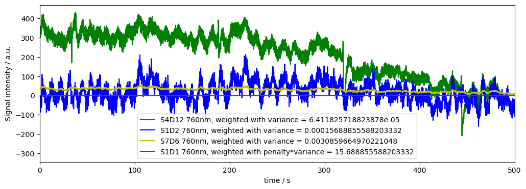
Lets apply this now, for instance to normalize signals using the noise proxy (smaller variance will amplify a signal)
[11]:
# normalize signals by their variance
rec["normalized_od"] = rec["od"] / od_var

# Plot normalized data for visual validation
f,ax = plt.subplots(1,1, figsize=(12,4))

ax.plot( rec["normalized_od"].time, rec["normalized_od"].sel(channel="S4D12", wavelength="760"), "g-", label="S4D12 760nm, weighted with variance = " +str(od_var.sel(channel="S4D12", wavelength="760").values))
ax.plot( rec["normalized_od"].time, rec["normalized_od"].sel(channel="S1D2", wavelength="760"), "b-", label="S1D2 760nm, weighted with variance = " +str(od_var.sel(channel="S1D2", wavelength="760").values))
ax.plot( rec["normalized_od"].time, rec["normalized_od"].sel(channel="S7D6", wavelength="760"), "y-", label="S7D6 760nm, weighted with variance = " +str(od_var.sel(channel="S7D6", wavelength="760").values))
ax.plot( rec["normalized_od"].time, rec["normalized_od"].sel(channel="S1D1", wavelength="760"), "r-", label="S1D1 760nm, weighted with penalty*variance = "+str(bad_rel_var*od_var.sel(channel="S1D2", wavelength="760").values))
plt.legend()
ax.set_xlim(0, 500)
ax.set_xlabel("time / s")
ax.set_ylabel("Signal intensity / a.u.")
/home/runner/miniconda3/envs/cedalion/lib/python3.11/site-packages/xarray/core/variable.py:315: UnitStrippedWarning: The unit of the quantity is stripped when downcasting to ndarray.
  data = np.asarray(data)
[11]:
Text(0, 0.5, 'Signal intensity / a.u.')
Channel Covariance
Lastly, we might also be interested in channel covariance…
[12]:
# use the same function to calculate the covariance of the optical density measurements
list_bad_channels = ["S1D1", "S4D4"]
bad_rel_var = 10  # much smaller factor than the default just to highlight the effect

od_covar = quality.measurement_variance(rec["od"], list_bad_channels, bad_rel_var, calc_covariance=True)
display(od_covar)


# use log(Var) again because we penalized the bad channels with a large factor
fig, ax = plot_heatmap(od_covar, cov_wavelength=760.0, figsize=(10, 10))
plt.show()
/home/runner/miniconda3/envs/cedalion/lib/python3.11/site-packages/xarray/core/variable.py:315: UnitStrippedWarning: The unit of the quantity is stripped when downcasting to ndarray.
  data = np.asarray(data)
/home/runner/work/cedalion/cedalion/src/cedalion/sigproc/quality.py:1351: UnitStrippedWarning: The unit of the quantity is stripped when downcasting to ndarray.
  cov_matrix_2d[bad_diag_mask] = var_fill_value
<xarray.DataArray (wavelength: 2, channel1: 28, channel2: 28)> Size: 13kB
array([[[ 5.07913635e-02,  4.54744404e-02,  4.54744404e-02, ...,
          4.54744404e-02,  4.54744404e-02,  4.54744404e-02],
        [ 4.54744404e-02,  1.56895307e-04,  2.25402930e-04, ...,
          2.41759032e-04,  2.76216376e-04,  9.30600163e-05],
        [ 4.54744404e-02,  2.25402930e-04,  1.70386835e-03, ...,
          1.97784287e-03,  2.58856492e-03,  8.23036523e-04],
        ...,
        [ 4.54744404e-02,  2.41759032e-04,  1.97784287e-03, ...,
          2.44574695e-03,  3.15103727e-03,  9.96720477e-04],
        [ 4.54744404e-02,  2.76216376e-04,  2.58856492e-03, ...,
          3.15103727e-03,  4.40790796e-03,  1.29882713e-03],
        [ 4.54744404e-02,  9.30600163e-05,  8.23036523e-04, ...,
          9.96720477e-04,  1.29882713e-03,  4.22596282e-04]],

       [[ 5.07913635e-02,  3.75545503e-02,  3.75545503e-02, ...,
          3.75545503e-02,  3.75545503e-02,  3.75545503e-02],
        [ 3.75545503e-02,  2.74457056e-04,  1.35641691e-04, ...,
          7.18770124e-05, -4.56328395e-05, -5.28042107e-06],
        [ 3.75545503e-02,  1.35641691e-04,  9.47287815e-04, ...,
          1.17153622e-03,  1.66195394e-03,  4.17517769e-04],
        ...,
        [ 3.75545503e-02,  7.18770124e-05,  1.17153622e-03, ...,
          1.67907429e-03,  2.36092571e-03,  5.78806258e-04],
        [ 3.75545503e-02, -4.56328395e-05,  1.66195394e-03, ...,
          2.36092571e-03,  4.07060265e-03,  8.57699132e-04],
        [ 3.75545503e-02, -5.28042107e-06,  4.17517769e-04, ...,
          5.78806258e-04,  8.57699132e-04,  2.32311204e-04]]],
      shape=(2, 28, 28))
Coordinates:
  * wavelength  (wavelength) float64 16B 760.0 850.0
  * channel1    (channel1) object 224B 'S1D1' 'S1D2' 'S1D3' ... 'S8D8' 'S8D16'
  * channel2    (channel2) object 224B 'S1D1' 'S1D2' 'S1D3' ... 'S8D8' 'S8D16'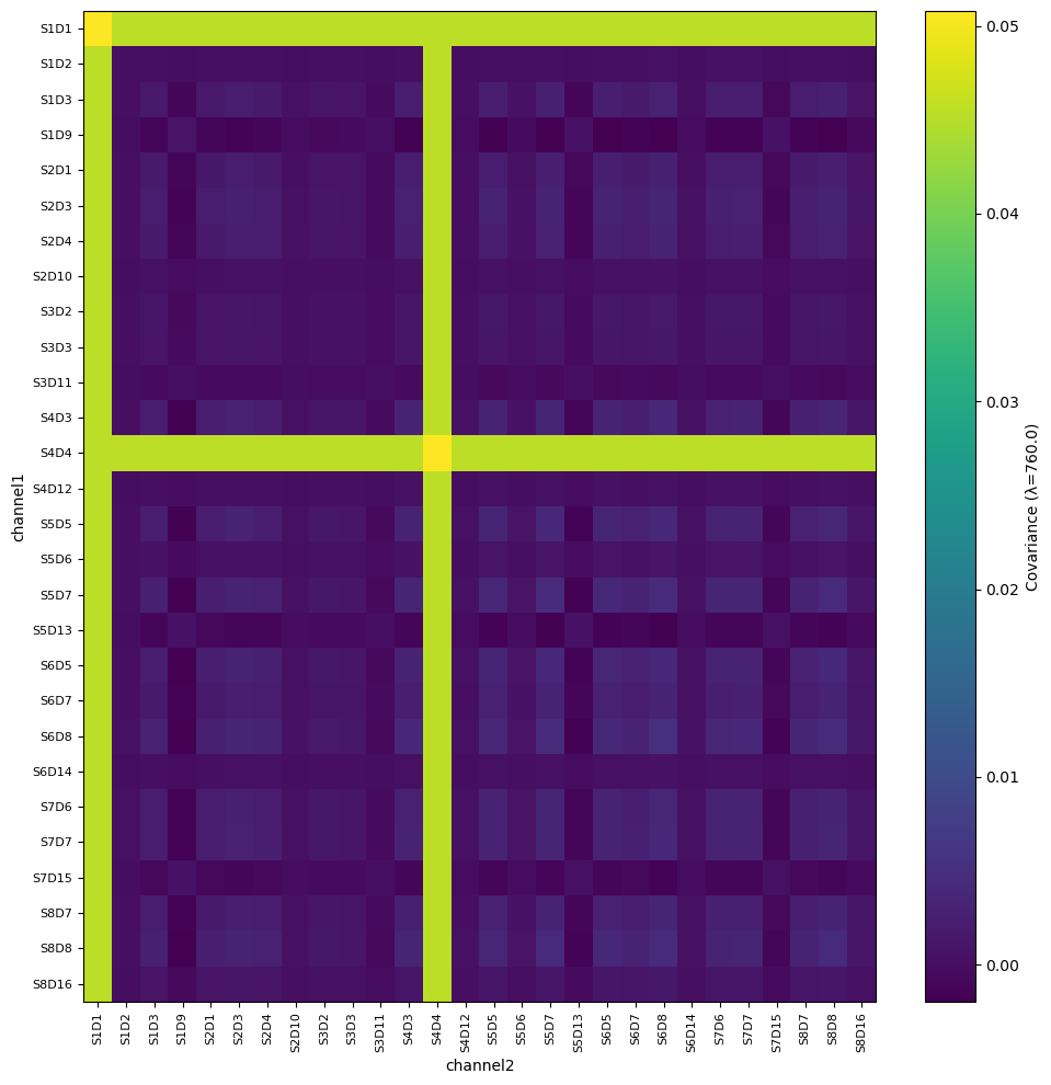
(Weighted) Global Physiology Removal
[13]:
from cedalion.sigproc.physio import global_component_subtract
[14]:
import xarray as xr

# just another helper function to make the relevant things below easier to read
def plot_channel_wavelength(
    rec: xr.Dataset,
    dname: str,
    diff: dict,
    global_comp: xr.DataArray,
    channel: str,
    wavelength: float
):
    f, ax = plt.subplots(1, 1, figsize=(12, 4))

    # Original signal
    ax.plot(
        rec["od"].time,
        rec["od"].sel({ "channel": channel, "wavelength": wavelength }),
        "b-",
        label=f"{channel} {wavelength}nm (raw)"
    )

    # Corrected signal
    ax.plot(
        rec[dname].time,
        rec[dname].sel({ "channel": channel, "wavelength": wavelength }),
        "g-",
        label=f"{channel} {wavelength}nm (corrected)"
    )

    # Global component
    ax.plot(
        global_comp.time,
        global_comp.sel({ "wavelength": wavelength }),
        "y-",
        label=f"Global Component {wavelength}nm"
    )

    # Difference (raw – corrected)
    ax.plot(
        rec["od"].time,
        diff[dname].sel({ "channel": channel, "wavelength": wavelength }),
        "r-",
        label="Difference (raw − corrected)"
    )

    ax.legend()
    ax.set_xlim(100, 200)
    ax.set_xlabel("time / s")
    ax.set_ylabel("Signal intensity / a.u.")
    plt.show()
First we get the original data and highpass filter it to remove slow drifts
[15]:
from cedalion.sigproc import frequency

# Refresh Data
rec["od"] = cedalion.nirs.cw.int2od(rec["amp"])

# highpass filter data to remove slow drifts
rec["od"] = frequency.freq_filter(rec["od"], fmin=0.01*units.Hz, fmax=2*units.Hz, butter_order=4)

# initialize empty dictionary
diff = {}
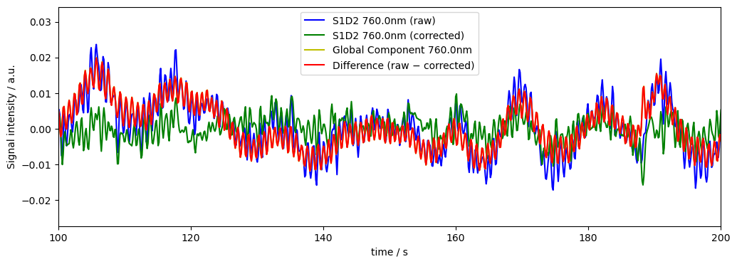
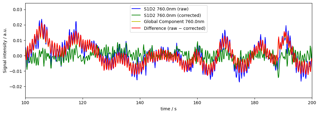
(Fitted) Global Mean Subtraction
We can use global_physio_subtract to remove the global average signal from each channel/vertex/voxel.
[16]:
dname = "od_corr_gm"

rec[dname], global_comp = global_component_subtract(rec["od"], ts_weights=None, k=0)
diff[dname] = rec["od"] - rec[dname]


# plot results for channel S1D2 at 760nm
plot_channel_wavelength(
    rec=rec,
    dname=dname,
    diff=diff,
    global_comp=global_comp,
    channel="S1D2",
    wavelength=760.0
)
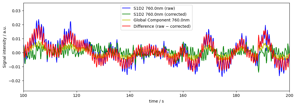
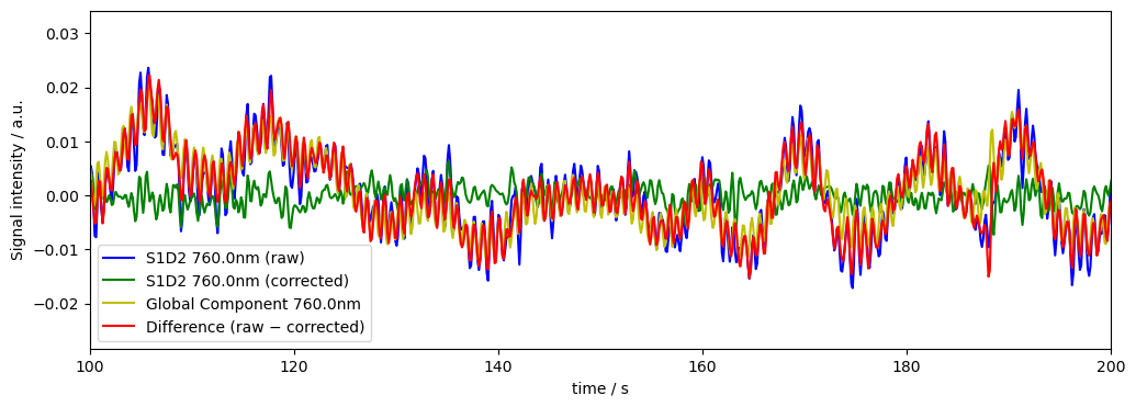
Weighted Global Mean Subtraction
Since some channels might have a lot of artifacts or are noisy, we can use the variance as proxy for channel measurement noise from above in this notebook, to downweight noisy channel in the global mean subtraction
[17]:
od_var = quality.measurement_variance(rec["od"], calc_covariance=False)

dname = "od_corr_wgm"
rec[dname], global_comp = global_component_subtract(rec["od"], ts_weights=1/od_var, k=0)
diff[dname] = rec["od"] - rec[dname]


# plot results for channel S1D2 at 760nm
plot_channel_wavelength(
    rec=rec,
    dname=dname,
    diff=diff,
    global_comp=global_comp,
    channel="S1D2",
    wavelength=760.0
)
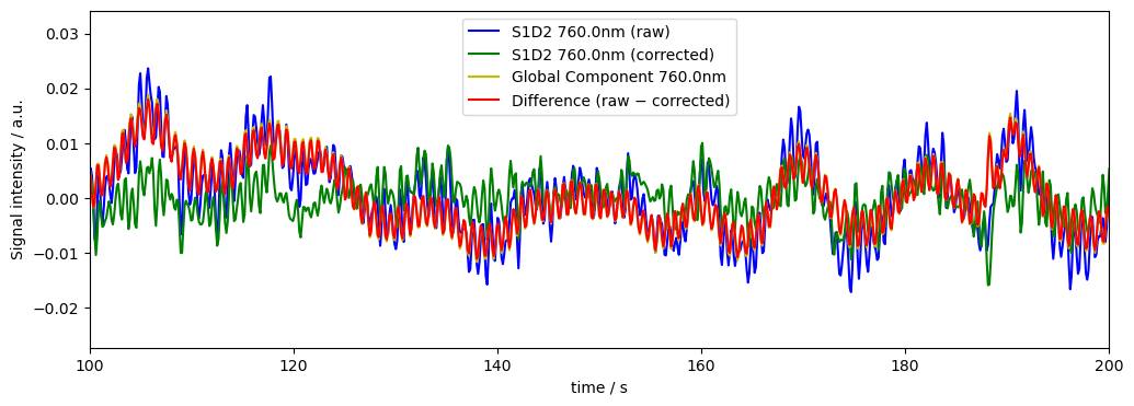
Remove exactly the first Principal Component (unweighted)
Instead of the global mean we can also use PCA to find and remove global components.
[18]:
dname = "od_corr_1pc"
rec[dname], global_comp = global_component_subtract(rec["od"], ts_weights=None, k=1)
diff[dname] = rec["od"] - rec[dname]


# plot results for channel S1D2 at 760nm
plot_channel_wavelength(
    rec=rec,
    dname=dname,
    diff=diff,
    global_comp=global_comp,
    channel="S1D2",
    wavelength=760.0
)
Remove 1 PCA component but using measurement‐variance weights on the data
If we want we can also include the channel weights from above in the PCA-based global signal removal
[19]:
od_var = quality.measurement_variance(rec["od"], calc_covariance=False)
dname = "od_corr_w1pc"

rec[dname], global_comp = global_component_subtract(rec["od"], ts_weights= 1/od_var, k=1)
diff[dname] = rec["od"] - rec[dname]

# plot results for channel S1D2 at 760nm
plot_channel_wavelength(
    rec=rec,
    dname=dname,
    diff=diff,
    global_comp=global_comp,
    channel="S1D2",
    wavelength=760.0
)
Remove 95% of global variance (weighted)
Often we dont know how many components to remove exactly, but how much variance the components we want to remove should explain. We can use k<1 to indicate the percent of variance we want removed.
[20]:
dname = "od_corr_w0.95pc"
rec[dname], global_comp = global_component_subtract(rec["od"], ts_weights=1/od_var, k=0.95)
diff[dname] = rec["od"] - rec[dname]


# plot results for channel S1D2 at 760nm
plot_channel_wavelength(
    rec=rec,
    dname=dname,
    diff=diff,
    global_comp=global_comp,
    channel="S1D2",
    wavelength=760.0
)
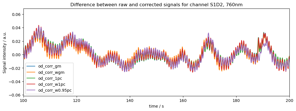
Overall comparison of the effects of the shown approaches
Lastly lets look at the difference (raw-corrected) signals for all of the approaches. Note that the differences between methods can be much stronger for more noisy data (our dataset here is quite clean)
[21]:
# plots all signals for channel S1D2, 760nm in diff[dname] for all dnames and puts the dnames in the legend

f, ax = plt.subplots(1, 1, figsize=(12,4))

for dname in diff.keys():
    ax.plot(
        rec["od"].time,
        diff[dname].sel({ "channel": "S7D6", "wavelength": 760.0 }),
        label=dname
    )
ax.set_title("Difference between raw and corrected signals for channel S1D2, 760nm")
ax.legend()
ax.set_xlim(100, 200)
ax.set_xlabel("time / s")
ax.set_ylabel("Signal intensity / a.u.")
plt.show()
References
[22]:
cedalion.bib.dump_to_notebook()
Methods used
| [1] | Luke2021 | cedalion.data.get_fingertapping | Robert Luke and David McAlpine. fNIRS Finger Tapping Data in BIDS Format. September 2021. doi:10.5281/zenodo.5529797. |
| [2] | Tucker2022 | cedalion.io.snirf.read_snirf | Stephen Tucker, Jay Dubb, Sreekanth Kura, Alexander von Lühmann, Robert Franke, Jörn M. Horschig, Samuel Powell, Robert Oostenveld, Michael Lührs, Édouard Delaire, Zahra M. Aghajan, Hanseok Yun, Meryem A. Yücel, Qianqian Fang, Theodore J. Huppert, Blaise deB. Frederick, Luca Pollonini, David A. Boas, and Robert Luke. Introduction to the shared near infrared spectroscopy format. Neurophotonics, 10(1):013507, 2022. doi:10.1117/1.NPh.10.1.013507. |
| [3] | Delpy1988 | cedalion.nirs.cw.int2od | D. T. Delpy, M. Cope, P. van der Zee, S. Arridge, S. Wray, and J. Wyatt. Estimation of optical pathlength through tissue from direct time of flight measurement. Physics in Medicine and Biology, 33(12):1433–1442, 1988. doi:10.1088/0031-9155/33/12/008. |
| [4] | Villringer1997 | cedalion.nirs.cw.int2od | Arno Villringer and Britton Chance. Non-invasive optical spectroscopy and imaging of human brain function. Trends in Neurosciences, 20(10):435–442, 1997. doi:10.1016/S0166-2236(97)01132-6. |
| [5] | Fishburn2019 | cedalion.sigproc.motion.tddr | Frank A. Fishburn, Ruth S. Ludlum, Chandan J. Vaidya, and Andrei V. Medvedev. Temporal derivative distribution repair (tddr): a motion correction method for fnirs. NeuroImage, 184:171–179, 2019. doi:https://doi.org/10.1016/j.neuroimage.2018.09.025. |
| [6] | Fishburn2018 | cedalion.sigproc.motion.tddr | Frank Fishburn. Tddr. 2018. URL: https://github.com/frankfishburn/TDDR/. |
| [7] | Molavi2012 | cedalion.sigproc.motion.wavelet | Behnam Molavi and Guy A Dumont. Wavelet-based motion artifact removal for functional near-infrared spectroscopy. Physiological Measurement, 33(2):259, 2012. doi:10.1088/0967-3334/33/2/259. |
| [8] | Huppert2009 | cedalion.sigproc.motion.wavelet | Theodore J. Huppert, Solomon G. Diamond, Maria A. Franceschini, and David A. Boas. Homer: a review of time-series analysis methods for near-infrared spectroscopy of the brain. Appl. Opt., 48(10):D280–D298, Apr 2009. doi:https://doi.org/10.1364/AO.48.00D280. |