Data Loading and Preprocessing
[1]:
# This cells setups the environment when executed in Google Colab.
try:
    import google.colab
    !curl -s https://raw.githubusercontent.com/ibs-lab/cedalion/dev/scripts/colab_setup.py -o colab_setup.py
    # Select branch with --branch "branch name" (default is "dev")
    %run colab_setup.py
except ImportError:
    pass
[2]:
import matplotlib.pyplot as p
import numpy as np

import cedalion
import cedalion.data
import cedalion.sigproc.motion as motion
import cedalion.sigproc.quality as quality
import cedalion.vis.blocks as vbx
import cedalion.vis.colors as colors
from cedalion.vis.anatomy import scalp_plot
from cedalion.vis.quality import plot_quality_mask
from cedalion import units
from cedalion.vis.anatomy import plot_montage3D
Load Data
Example datasets are accessible through functions in cedalion.data. These take care of downloading, caching and updating the data files. Often they also already load the data.
Here we load a single-subject DOT dataset with a motor task.
[3]:
rec = cedalion.data.get_fingertappingDOT()
This recording object hold a single NIRS time series 'amp'
[4]:
rec.timeseries.keys()
[4]:
odict_keys(['amp'])
It contains several auxiliary time series from additional sensors:
[5]:
rec.aux_ts.keys()
[5]:
odict_keys(['ACCEL_X_1', 'ACCEL_Y_1', 'ACCEL_Z_1', 'GYRO_X_1', 'GYRO_Y_1', 'GYRO_Z_1', 'ExGa1', 'ExGa2', 'ExGa3', 'ExGa4', 'ECG', 'Respiration', 'PPG', 'SpO2', 'Heartrate', 'GSR', 'Temperature'])
Inspecting the Datasets
Raw Amplitude Time Series
[6]:
rec["amp"]
[6]:
<xarray.DataArray (channel: 100, wavelength: 2, time: 8794)> Size: 14MB
<Quantity([[[0.08740092 0.08734962 0.08818625 ... 0.09035587 0.09098899 0.09272738]
  [0.13985697 0.13982265 0.14141524 ... 0.13390421 0.13521901 0.13864038]]

 [[0.27071937 0.27030255 0.27172273 ... 0.26408907 0.26584981 0.26889485]
  [0.65636219 0.65455566 0.65930072 ... 0.62508687 0.63123411 0.64150497]]

 [[0.12522511 0.1251687  0.12585573 ... 0.1244254  0.1247638  0.12649158]
  [0.20260527 0.2023983  0.20387637 ... 0.19096156 0.19242489 0.19605342]]

 ...

 [[0.12742799 0.12771832 0.12856142 ... 0.12475135 0.1240544  0.1230771 ]
  [0.28363299 0.28471081 0.2877631  ... 0.26401558 0.26345736 0.26146422]]

 [[0.03967372 0.03983601 0.04008131 ... 0.03961476 0.03932456 0.03901398]
  [0.1705261  0.17133473 0.17316591 ... 0.16186236 0.16202994 0.16063383]]

 [[0.08932346 0.08954745 0.0901911  ... 0.08869942 0.08842191 0.08802665]
  [0.09587179 0.09623634 0.09746928 ... 0.09036516 0.09042745 0.08998772]]], 'volt')>
Coordinates:
  * time        (time) float64 70kB 0.0 0.2294 0.4588 ... 2.017e+03 2.017e+03
    samples     (time) int64 70kB 0 1 2 3 4 5 ... 8788 8789 8790 8791 8792 8793
  * channel     (channel) object 800B 'S1D1' 'S1D2' 'S1D4' ... 'S14D31' 'S14D32'
    source      (channel) object 800B 'S1' 'S1' 'S1' 'S1' ... 'S14' 'S14' 'S14'
    detector    (channel) object 800B 'D1' 'D2' 'D4' 'D5' ... 'D29' 'D31' 'D32'
  * wavelength  (wavelength) float64 16B 760.0 850.0
Attributes:
data_type_group: unprocessed rawStimulus event information
[7]:
rec.stim
[7]:
| onset | duration | value | trial_type | |
|---|---|---|---|---|
| 0 | 23.855104 | 10.0 | 1.0 | 1 |
| 1 | 54.132736 | 10.0 | 1.0 | 1 |
| 2 | 84.410368 | 10.0 | 1.0 | 1 |
| 3 | 114.688000 | 10.0 | 1.0 | 1 |
| 4 | 146.112512 | 10.0 | 1.0 | 1 |
| ... | ... | ... | ... | ... |
| 125 | 1431.535616 | 10.0 | 1.0 | 5 |
| 126 | 1526.038528 | 10.0 | 1.0 | 5 |
| 127 | 1650.819072 | 10.0 | 1.0 | 5 |
| 128 | 1805.418496 | 10.0 | 1.0 | 5 |
| 129 | 1931.116544 | 10.0 | 1.0 | 5 |
130 rows × 4 columns
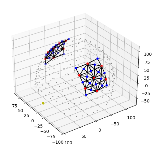
Montage
[8]:
rec.geo3d
[8]:
<xarray.DataArray (label: 346, digitized: 3)> Size: 8kB
<Quantity([[-77.817871  15.680614  23.17227 ]
 [-61.906841  21.227732  56.492802]
 [-85.37146  -16.079958   8.900885]
 ...
 [ 77.521     28.883    -39.113   ]
 [ 80.59      14.229    -38.278   ]
 [ 81.95      -0.678    -37.027   ]], 'millimeter')>
Coordinates:
    type     (label) object 3kB PointType.SOURCE ... PointType.LANDMARK
  * label    (label) <U6 8kB 'S1' 'S2' 'S3' 'S4' ... 'FFT10h' 'FT10h' 'FTT10h'
Dimensions without coordinates: digitized[9]:
plot_montage3D(rec["amp"], rec.geo3d)
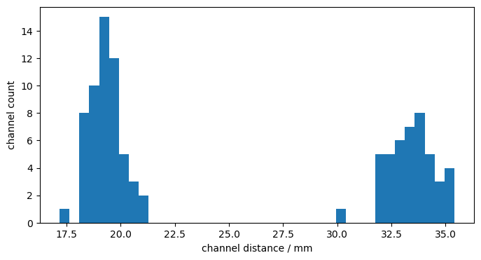
Channel Distances
[10]:
distances = cedalion.nirs.channel_distances(rec["amp"], rec.geo3d)

p.figure(figsize=(8,4))
p.hist(distances, 40)
p.xlabel("channel distance / mm")
p.ylabel("channel count");
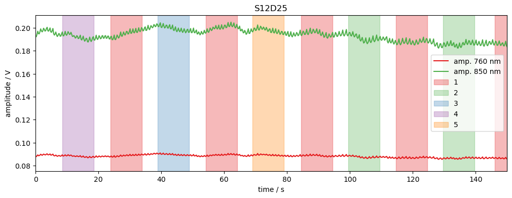
Plot raw amplitude for one channel
[11]:
# example time trace
amp = rec["amp"]
ch = "S12D25"
f, ax = p.subplots(1,1, figsize=(12,4))
ax.set_prop_cycle("color", colors.COLORBREWER_Q8)
ax.plot(amp.time, amp.sel(channel=ch, wavelength=760), label="amp. 760 nm")
ax.plot(amp.time, amp.sel(channel=ch, wavelength=850), label="amp. 850 nm")
vbx.plot_stim_markers(ax, rec.stim, y=1)
ax.set_xlabel("time / s")
ax.set_ylabel("amplitude / V")
ax.set_xlim(0,150)
ax.legend()
ax.set_title(ch);
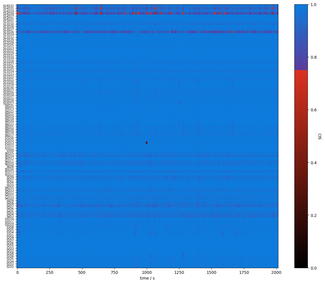
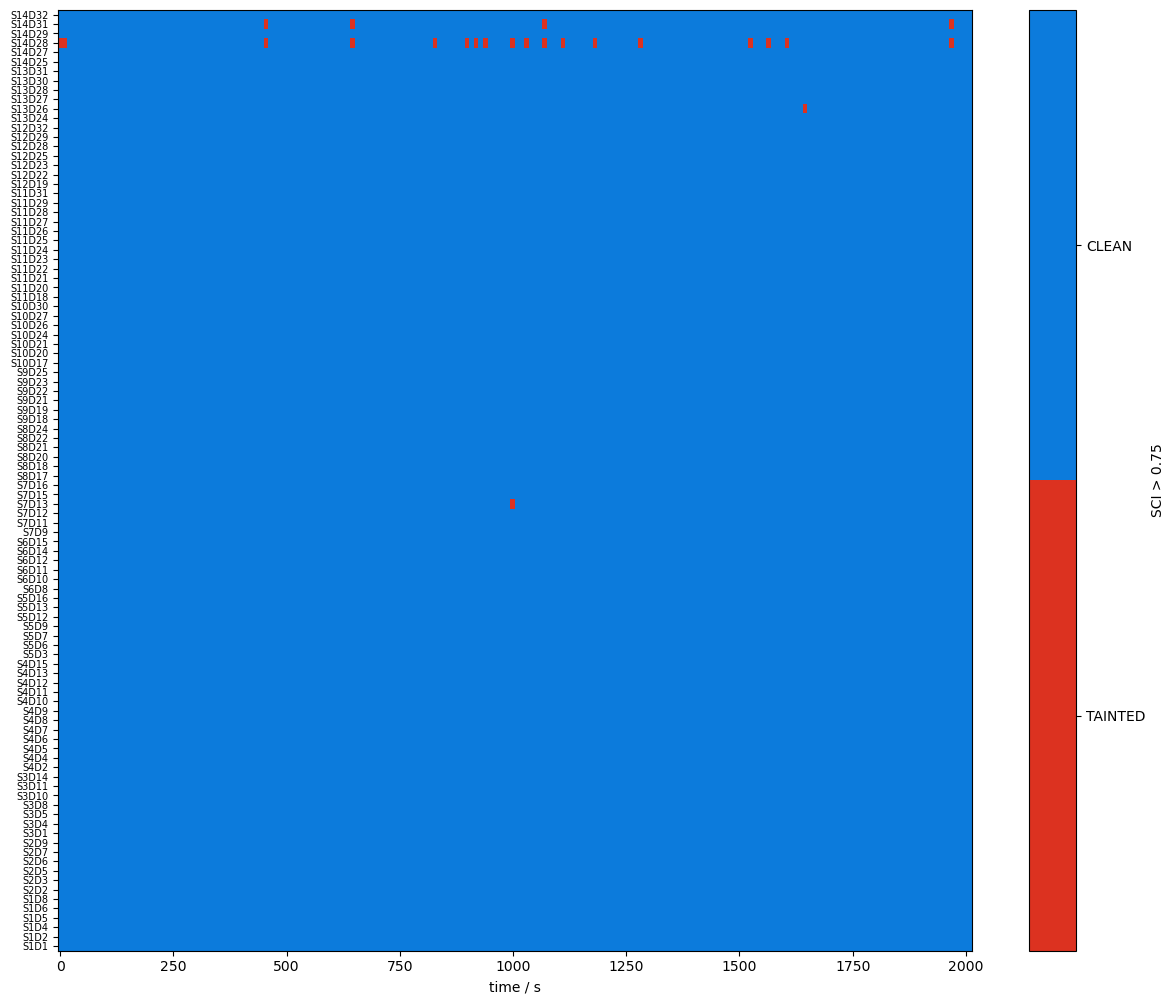
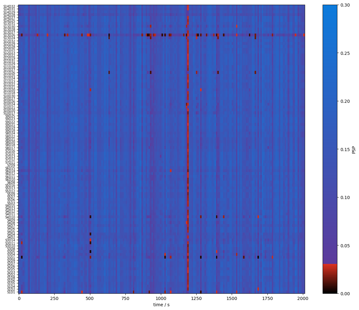
Quality Metrics : SCI & PSP
using functions from cedalion.sigproc.quality we calculate two metrics:
scalp coupling index (SCI)
peak spectral power (PSP)
note the different time axis: both metrics a calculated in sliding windows
both functions return a metric and boolean arrays (masks) if the metric is above threshold
[12]:
sci_threshold = 0.75
window_length = 10*units.s
sci, sci_mask = quality.sci(rec["amp"], window_length, sci_threshold)
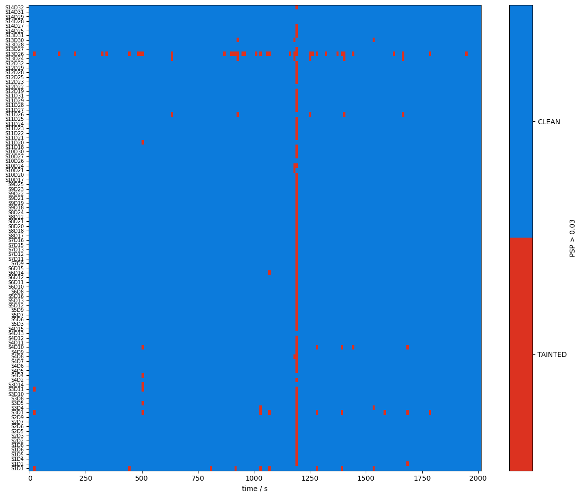
psp_threshold = 0.03
psp, psp_mask = quality.psp(rec["amp"], window_length, psp_threshold)
display(sci.rename("sci"))
display(sci_mask.rename("sci_mask"))
<xarray.DataArray 'sci' (channel: 100, time: 200)> Size: 160kB
array([[0.9949109 , 0.9949109 , 0.97750268, ..., 0.99755867, 0.99673787,
        0.99561847],
       [0.99159096, 0.99159096, 0.93520281, ..., 0.99238156, 0.99570154,
        0.98828878],
       [0.99206498, 0.99206498, 0.9939492 , ..., 0.99527559, 0.99615776,
        0.99315244],
       ...,
       [0.94375225, 0.94375225, 0.95649474, ..., 0.95639974, 0.97469584,
        0.92564555],
       [0.86450677, 0.86450677, 0.91515934, ..., 0.94323422, 0.94480114,
        0.87333273],
       [0.96496945, 0.96496945, 0.97428204, ..., 0.96280239, 0.97176867,
        0.95451752]], shape=(100, 200))
Coordinates:
  * time      (time) float64 2kB 0.0 10.09 20.19 ... 1.998e+03 2.008e+03
    samples   (time) int64 2kB 0 44 88 132 176 220 ... 8580 8624 8668 8712 8756
  * channel   (channel) object 800B 'S1D1' 'S1D2' 'S1D4' ... 'S14D31' 'S14D32'
    source    (channel) object 800B 'S1' 'S1' 'S1' 'S1' ... 'S14' 'S14' 'S14'
detector (channel) object 800B 'D1' 'D2' 'D4' 'D5' ... 'D29' 'D31' 'D32'<xarray.DataArray 'sci_mask' (channel: 100, time: 200)> Size: 20kB
array([[ True,  True,  True, ...,  True,  True,  True],
       [ True,  True,  True, ...,  True,  True,  True],
       [ True,  True,  True, ...,  True,  True,  True],
       ...,
       [ True,  True,  True, ...,  True,  True,  True],
       [ True,  True,  True, ...,  True,  True,  True],
       [ True,  True,  True, ...,  True,  True,  True]], shape=(100, 200))
Coordinates:
* time (time) float64 2kB 0.0 10.09 20.19 ... 1.998e+03 2.008e+03
samples (time) int64 2kB 0 44 88 132 176 220 ... 8580 8624 8668 8712 8756
* channel (channel) object 800B 'S1D1' 'S1D2' 'S1D4' ... 'S14D31' 'S14D32'
source (channel) object 800B 'S1' 'S1' 'S1' 'S1' ... 'S14' 'S14' 'S14'
detector (channel) object 800B 'D1' 'D2' 'D4' 'D5' ... 'D29' 'D31' 'D32'[13]:
# define three colomaps: redish below a threshold, blueish above
sci_norm, sci_cmap = colors.threshold_cmap("sci_cmap", 0., 1.0, sci_threshold)
psp_norm, psp_cmap = colors.threshold_cmap("psp_cmap", 0., 0.30, psp_threshold)

def plot_sci(sci):
    # plot the heatmap
    f,ax = p.subplots(1,1,figsize=(12,10))

    m = ax.pcolormesh(sci.time, np.arange(len(sci.channel)), sci, shading="nearest", cmap=sci_cmap, norm=sci_norm)
    cb = p.colorbar(m, ax=ax)
    cb.set_label("SCI")
    ax.set_xlabel("time / s")
    p.tight_layout()
    ax.yaxis.set_ticks(np.arange(len(sci.channel)))
    ax.yaxis.set_ticklabels(sci.channel.values, fontsize=7)

def plot_psp(psp):
    f,ax = p.subplots(1,1,figsize=(12,10))

    m = ax.pcolormesh(psp.time, np.arange(len(psp.channel)), psp, shading="nearest", cmap=psp_cmap, norm=psp_norm)
    cb = p.colorbar(m, ax=ax)
    cb.set_label("PSP")
    ax.set_xlabel("time / s")
    p.tight_layout()
    ax.yaxis.set_ticks(np.arange(len(psp.channel)))
    ax.yaxis.set_ticklabels(psp.channel.values, fontsize=7)
[14]:
plot_sci(sci)
plot_quality_mask(sci > sci_threshold, f"SCI > {sci_threshold}")
plot_psp(psp)
plot_quality_mask(psp > psp_threshold, f"PSP > {psp_threshold}")
Combining Signal Quality Masks
We want both SCI and PSP to be above their respective thresholds for a window to be considered clean. We can use the boolean and operation to combine both and then look at the percentage of time both metrics are above the thresholds.
[15]:
combined_mask = sci_mask & psp_mask

display(combined_mask)
plot_quality_mask(combined_mask, "combined_mask")
<xarray.DataArray (channel: 100, time: 200)> Size: 20kB
array([[ True,  True, False, ...,  True,  True,  True],
       [ True,  True,  True, ...,  True,  True,  True],
       [ True,  True,  True, ...,  True,  True,  True],
       ...,
       [ True,  True,  True, ...,  True,  True,  True],
       [ True,  True,  True, ...,  True,  True,  True],
       [ True,  True,  True, ...,  True,  True,  True]], shape=(100, 200))
Coordinates:
  * time      (time) float64 2kB 0.0 10.09 20.19 ... 1.998e+03 2.008e+03
    samples   (time) int64 2kB 0 44 88 132 176 220 ... 8580 8624 8668 8712 8756
  * channel   (channel) object 800B 'S1D1' 'S1D2' 'S1D4' ... 'S14D31' 'S14D32'
    source    (channel) object 800B 'S1' 'S1' 'S1' 'S1' ... 'S14' 'S14' 'S14'
    detector  (channel) object 800B 'D1' 'D2' 'D4' 'D5' ... 'D29' 'D31' 'D32'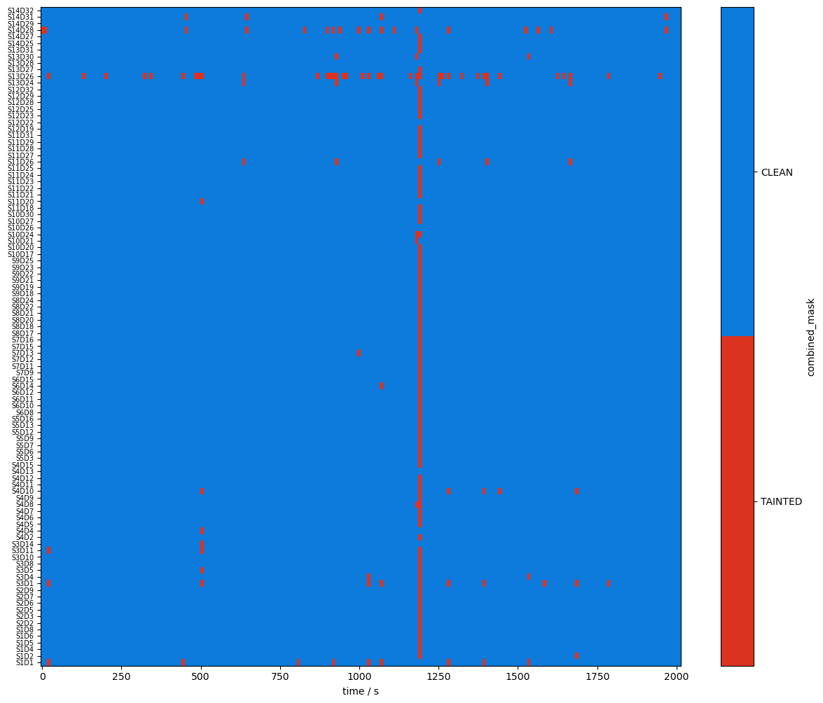
calculate percentage of clean time per channel
[16]:
perc_time_clean = combined_mask.sum(dim="time") / len(sci.time)

display(perc_time_clean)

f, ax = p.subplots(1,1,figsize=(6.5,6.5))

scalp_plot(
    rec["amp"],
    rec.geo3d,
    perc_time_clean,
    ax,
    cmap="RdYlGn",
    vmin=0.80,
    vmax=1,
    title=None,
    cb_label="Percentage of clean time",
    channel_lw=2,
    optode_labels=True
)
f.tight_layout()
<xarray.DataArray (channel: 100)> Size: 800B
array([0.955, 0.99 , 0.995, 0.995, 0.995, 0.995, 0.995, 0.995, 0.995,
       0.995, 0.995, 0.995, 0.95 , 0.985, 0.99 , 0.995, 0.995, 0.985,
       0.995, 0.995, 0.995, 0.995, 0.995, 0.995, 0.99 , 0.995, 0.97 ,
       0.995, 0.995, 1.   , 0.995, 0.995, 0.995, 0.995, 0.995, 0.995,
       0.995, 0.995, 0.995, 0.995, 0.995, 0.995, 0.99 , 0.995, 0.995,
       0.995, 0.995, 0.99 , 0.995, 0.995, 0.995, 0.995, 0.995, 0.995,
       0.995, 0.995, 0.995, 0.995, 0.995, 0.995, 0.995, 0.995, 0.995,
       0.995, 0.995, 0.99 , 1.   , 0.995, 0.995, 0.995, 0.995, 0.995,
       0.995, 0.995, 0.995, 0.995, 0.975, 0.995, 0.995, 0.995, 0.995,
       0.995, 1.   , 0.995, 0.995, 0.995, 0.995, 0.995, 0.97 , 0.815,
       0.995, 1.   , 0.985, 0.995, 0.995, 0.995, 0.91 , 1.   , 0.98 ,
       0.995])
Coordinates:
  * channel   (channel) object 800B 'S1D1' 'S1D2' 'S1D4' ... 'S14D31' 'S14D32'
    source    (channel) object 800B 'S1' 'S1' 'S1' 'S1' ... 'S14' 'S14' 'S14'
    detector  (channel) object 800B 'D1' 'D2' 'D4' 'D5' ... 'D29' 'D31' 'D32'
Correct Motion Artefacts
use
cedalion.nirs.cw.int2odto get optical densitiesapply Temporal Derivative Distribution Repair (TDDR) first to correct jumps
then apply Wavelet motion artifact correction
[17]:
rec["od"] = cedalion.nirs.cw.int2od(rec["amp"])
rec["od_tddr"] = motion.tddr(rec["od"])
rec["od_wavelet"] = motion.wavelet(rec["od_tddr"])
rec["amp_corrected"] = cedalion.nirs.cw.od2int(rec["od_wavelet"], rec["amp"].mean("time"))
[18]:
# recalculate sci & psp on cleaned data
sci_corr, sci_corr_mask = quality.sci(rec["amp_corrected"], window_length, sci_threshold)
psp_corr, psp_corr_mask = quality.psp(rec["amp_corrected"], window_length, psp_threshold)
combined_corr_mask = sci_corr_mask & psp_corr_mask
[19]:
plot_quality_mask(combined_mask, f"combined mask")
plot_quality_mask(combined_corr_mask, f"combined corrected mask")


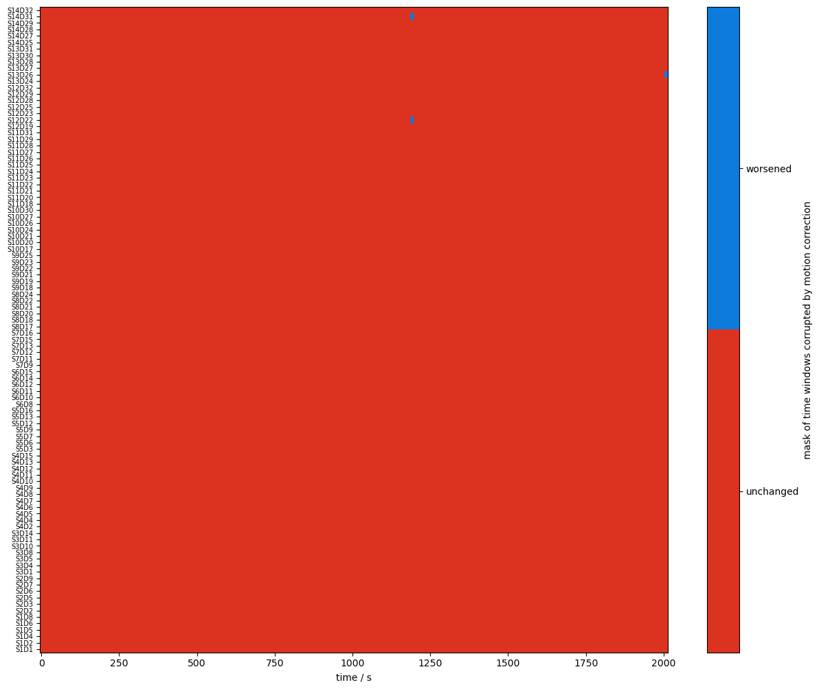
Compare masks before and after motion artifact correction
[20]:
changed_windows = (combined_mask == quality.TAINTED) & (combined_corr_mask == quality.CLEAN)

plot_quality_mask(changed_windows, "mask of time windows cleaned by motion correction", bool_labels=["unchanged", "improved"])

changed_windows = (combined_mask == quality.CLEAN) & (combined_corr_mask == quality.TAINTED)

plot_quality_mask(changed_windows, "mask of time windows corrupted by motion correction", bool_labels=["unchanged", "worsened"])

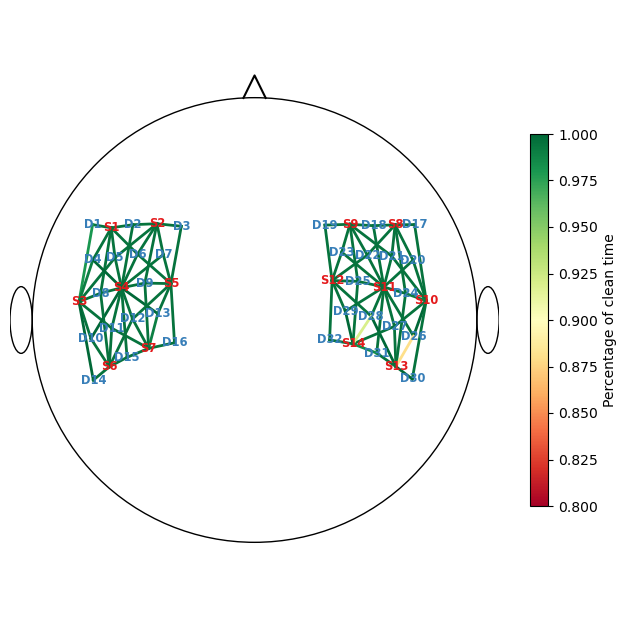
recalculate percentage of clean time
[21]:
perc_time_clean_corr = combined_corr_mask.sum(dim="time") / len(sci.time)

f, ax = p.subplots(1,1,figsize=(6.5,6.5))

scalp_plot(
    rec["amp"],
    rec.geo3d,
    perc_time_clean_corr,
    ax,
    cmap="RdYlGn",
    vmin=0.80,
    vmax=1,
    title=None,
    cb_label="Percentage of clean time",
    channel_lw=2,
    optode_labels=True
)
f.tight_layout()
Global Variance of the Temporal Derivative (GVTD) for identifying global bad time segments
[22]:
gvtd, gvtd_mask = quality.gvtd(rec["amp"])
gvtd_corr, gvtd_prr_mask = quality.gvtd(rec["amp_corrected"])
[23]:
# select the 10 segments with highest gvtd
top10_bad_segments = sorted(
    [seg for seg in quality.mask_to_segments(combined_mask.all("channel"))],
    key=lambda t: gvtd.sel(time=slice(t[0], t[1])).max(),
    reverse=True,
)[:10]
Calculate GVTD for the original and corrected time series
[24]:
f,ax = p.subplots(4,1,figsize=(16,6), sharex=True)
ax[0].plot(gvtd.time, gvtd)
ax[1].plot(combined_mask.time, combined_mask.all("channel"))
ax[2].plot(gvtd_corr.time, gvtd_corr)
ax[3].plot(combined_corr_mask.time, combined_corr_mask.all("channel"))
ax[0].set_ylim(0, 0.02)
ax[2].set_ylim(0, 0.02)
ax[0].set_ylabel("GVTD")
ax[2].set_ylabel("GVTD")
ax[1].set_ylabel("combined_mask")
ax[3].set_ylabel("combined_corr_mask")
ax[3].set_xlabel("time / s")

for i in range(4):
    vbx.plot_segments(ax[i], top10_bad_segments)

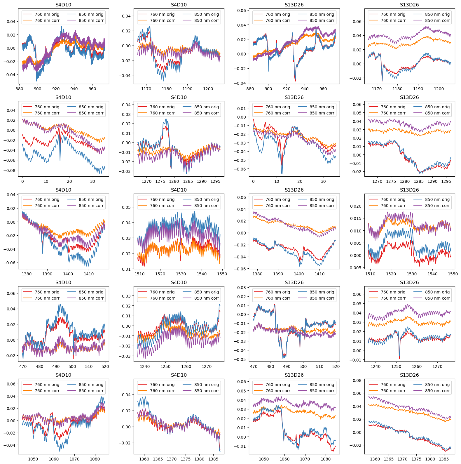
Highlight motion correction in selected segments
[25]:
example_channels = ["S4D10", "S13D26"]

f, ax = p.subplots(5,4, figsize=(16,16), sharex=False)
ax = ax.T.flatten()
padding = 15
i = 0
for ch in example_channels:
    for (start, end) in top10_bad_segments:
        ax[i].set_prop_cycle(color=["#e41a1c", "#ff7f00", "#377eb8", "#984ea3"])
        for wl in rec["od"].wavelength.values:
            sel = rec["od"].sel(time=slice(start-padding, end+padding), channel=ch, wavelength=wl)
            ax[i].plot(sel.time, sel, label=f"{wl:.0f} nm orig")
            sel = rec["od_wavelet"].sel(time=slice(start-padding, end+padding), channel=ch, wavelength=wl)
            ax[i].plot(sel.time, sel, label=f"{wl:.0f} nm corr")
            ax[i].set_title(ch)
        ax[i].legend(ncol=2, loc="upper center")
        ylim = ax[i].get_ylim()
        ax[i].set_ylim(ylim[0], ylim[1]+0.25*(ylim[1]-ylim[0])) # make space for legend

        i += 1

p.tight_layout()
Final channel selection
[26]:
perc_time_clean_corr[perc_time_clean_corr < 0.95]
[26]:
<xarray.DataArray (channel: 2)> Size: 16B
array([0.88, 0.92])
Coordinates:
  * channel   (channel) object 16B 'S13D26' 'S14D28'
    source    (channel) object 16B 'S13' 'S14'
detector (channel) object 16B 'D26' 'D28'[27]:
signal_quality_selection_masks = [perc_time_clean >= .95]

rec["amp_pruned"], pruned_channels = quality.prune_ch(
    rec["amp"], signal_quality_selection_masks, "all"
)
display(rec["amp_pruned"])
display(pruned_channels)
<xarray.DataArray (channel: 98, wavelength: 2, time: 8794)> Size: 14MB
<Quantity([[[0.08740092 0.08734962 0.08818625 ... 0.09035587 0.09098899 0.09272738]
  [0.13985697 0.13982265 0.14141524 ... 0.13390421 0.13521901 0.13864038]]

 [[0.27071937 0.27030255 0.27172273 ... 0.26408907 0.26584981 0.26889485]
  [0.65636219 0.65455566 0.65930072 ... 0.62508687 0.63123411 0.64150497]]

 [[0.12522511 0.1251687  0.12585573 ... 0.1244254  0.1247638  0.12649158]
  [0.20260527 0.2023983  0.20387637 ... 0.19096156 0.19242489 0.19605342]]

 ...

 [[0.12742799 0.12771832 0.12856142 ... 0.12475135 0.1240544  0.1230771 ]
  [0.28363299 0.28471081 0.2877631  ... 0.26401558 0.26345736 0.26146422]]

 [[0.03967372 0.03983601 0.04008131 ... 0.03961476 0.03932456 0.03901398]
  [0.1705261  0.17133473 0.17316591 ... 0.16186236 0.16202994 0.16063383]]

 [[0.08932346 0.08954745 0.0901911  ... 0.08869942 0.08842191 0.08802665]
  [0.09587179 0.09623634 0.09746928 ... 0.09036516 0.09042745 0.08998772]]], 'volt')>
Coordinates:
  * time        (time) float64 70kB 0.0 0.2294 0.4588 ... 2.017e+03 2.017e+03
    samples     (time) int64 70kB 0 1 2 3 4 5 ... 8788 8789 8790 8791 8792 8793
  * channel     (channel) object 784B 'S1D1' 'S1D2' 'S1D4' ... 'S14D31' 'S14D32'
    source      (channel) object 784B 'S1' 'S1' 'S1' 'S1' ... 'S14' 'S14' 'S14'
    detector    (channel) object 784B 'D1' 'D2' 'D4' 'D5' ... 'D29' 'D31' 'D32'
  * wavelength  (wavelength) float64 16B 760.0 850.0
Attributes:
    data_type_group:  unprocessed raw
array(['S13D26', 'S14D28'], dtype=object)
References
[28]:
cedalion.bib.dump_to_notebook()
Methods used
| [1] | Tucker2022 | cedalion.io.snirf.read_snirf | Stephen Tucker, Jay Dubb, Sreekanth Kura, Alexander von Lühmann, Robert Franke, Jörn M. Horschig, Samuel Powell, Robert Oostenveld, Michael Lührs, Édouard Delaire, Zahra M. Aghajan, Hanseok Yun, Meryem A. Yücel, Qianqian Fang, Theodore J. Huppert, Blaise deB. Frederick, Luca Pollonini, David A. Boas, and Robert Luke. Introduction to the shared near infrared spectroscopy format. Neurophotonics, 10(1):013507, 2022. doi:10.1117/1.NPh.10.1.013507. |
| [2] | Pollonini2014 | cedalion.sigproc.quality.psp, cedalion.sigproc.quality.sci | Luca Pollonini, Cristen Olds, Homer Abaya, Heather Bortfeld, Michael S. Beauchamp, and John S. Oghalai. Auditory cortex activation to natural speech and simulated cochlear implant speech measured with functional near-infrared spectroscopy. Hearing Research, 309:84–93, 2014. doi:https://doi.org/10.1016/j.heares.2013.11.007. |
| [3] | Pollonini2016 | cedalion.sigproc.quality.psp, cedalion.sigproc.quality.sci | Luca Pollonini, Heather Bortfeld, and John S. Oghalai. PHOEBE: a method for real time mapping of optodes-scalp coupling in functional near-infrared spectroscopy. Biomedical Optics Express, 7(12):5104, Dec 2016. doi:10.1364/BOE.7.005104. |
| [4] | Delpy1988 | cedalion.nirs.cw.int2od | D. T. Delpy, M. Cope, P. van der Zee, S. Arridge, S. Wray, and J. Wyatt. Estimation of optical pathlength through tissue from direct time of flight measurement. Physics in Medicine and Biology, 33(12):1433–1442, 1988. doi:10.1088/0031-9155/33/12/008. |
| [5] | Villringer1997 | cedalion.nirs.cw.int2od | Arno Villringer and Britton Chance. Non-invasive optical spectroscopy and imaging of human brain function. Trends in Neurosciences, 20(10):435–442, 1997. doi:10.1016/S0166-2236(97)01132-6. |
| [6] | Fishburn2019 | cedalion.sigproc.motion.tddr | Frank A. Fishburn, Ruth S. Ludlum, Chandan J. Vaidya, and Andrei V. Medvedev. Temporal derivative distribution repair (tddr): a motion correction method for fnirs. NeuroImage, 184:171–179, 2019. doi:https://doi.org/10.1016/j.neuroimage.2018.09.025. |
| [7] | Fishburn2018 | cedalion.sigproc.motion.tddr | Frank Fishburn. Tddr. 2018. URL: https://github.com/frankfishburn/TDDR/. |
| [8] | Molavi2012 | cedalion.sigproc.motion.wavelet | Behnam Molavi and Guy A Dumont. Wavelet-based motion artifact removal for functional near-infrared spectroscopy. Physiological Measurement, 33(2):259, 2012. doi:10.1088/0967-3334/33/2/259. |
| [9] | Huppert2009 | cedalion.sigproc.motion.wavelet | Theodore J. Huppert, Solomon G. Diamond, Maria A. Franceschini, and David A. Boas. Homer: a review of time-series analysis methods for near-infrared spectroscopy of the brain. Appl. Opt., 48(10):D280–D298, Apr 2009. doi:https://doi.org/10.1364/AO.48.00D280. |
| [10] | Sherafati2020 | cedalion.sigproc.quality._get_gvtd_threshold, cedalion.sigproc.quality.gvtd | Arefeh Sherafati, Abraham Z. Snyder, Adam T. Eggebrecht, Karla M. Bergonzi, Tracy M. Burns-Yocum, Heather M. Lugar, Silvina L. Ferradal, Amy Robichaux-Viehoever, Christopher D. Smyser, Ben J. Palanca, Tamara Hershey, and Joseph P. Culver. Global motion detection and censoring in high-density diffuse optical tomography. Human Brain Mapping, 41(14):4093–4112, 2020. doi:https://doi.org/10.1002/hbm.25111. |