
Advanced single-trial fNIRS finger tapping classification
This notebook analyzes a multi-subject finger-tapping dataset and trains a Linear Discriminant Analysis (LDA) classifier to distinguish single trials of left-hand tapping from a resting/control condition.
Compared to the introductory 50_finger_tapping_lda_classification.ipynb notebook, this one goes into more depth:
Channels are pruned per subject using the Scalp Coupling Index (SCI) and Peak Spectral Power (PSP) quality metrics.
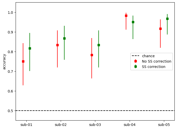
A GLM-based short-separation channel (SSC) regression is used to remove the systemic/superficial component from the long-channel concentration signal, and classification accuracy with and without this regression is compared via cross-validation.
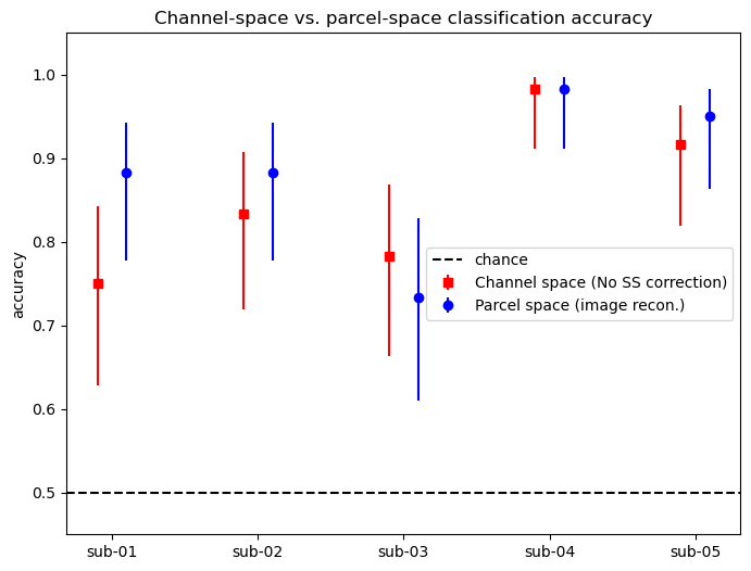
At the end of the notebook, the same trials are additionally analyzed in image (parcel) space: channel-space optical density is projected onto the cortical surface via diffuse optical tomography (DOT) image reconstruction, aggregated into brain parcels, and classified with the same features and classifier used for channel space — allowing a direct comparison of classification performance between channel-space and parcel-space representations.
On a basic level, this notebook illustrates some of the elements investigated more rigorously in [FMMvonLuhmann26], who show that single-trial fNIRS decoding accuracy improves systematically with higher optode density, model-based (GLM) noise regression, and image reconstruction. This notebook uses a single, comparatively sparse probe and a simple LDA classifier, so it should be read as a minimal illustration of the type of comparison made in that paper (channel space vs. image/parcel space, with/without regression), not as a reproduction of its results.
PLEASE NOTE: For simplicity’s sake we still skip several preprocessing steps that a rigorous analysis would include (e.g. motion artifact rejection beyond TDDR/wavelet correction, physiological noise regression beyond short-separation channels). These are the subject of other example notebooks. The purpose of this notebook is to demonstrate how cedalion interfaces with scikit-learn for both channel-space and image-space classification.
[1]:
# This cells setups the environment when executed in Google Colab.
try:
    import google.colab
    !curl -s https://raw.githubusercontent.com/ibs-lab/cedalion/dev/scripts/colab_setup.py -o colab_setup.py
    # Select branch with --branch "branch name" (default is "dev")
    %run colab_setup.py
except ImportError:
    pass
[2]:
from collections import defaultdict
import gc

import matplotlib.pyplot as p
import numpy as np
import pyvista as pv
import xarray as xr
from sklearn.discriminant_analysis import LinearDiscriminantAnalysis
from sklearn.pipeline import make_pipeline
from sklearn.preprocessing import LabelEncoder, StandardScaler

import cedalion
import cedalion.data
import cedalion.dot
import cedalion.geometry.landmarks
import cedalion.io
import cedalion.mlutils as mlutils
import cedalion.models.glm as glm
import cedalion.nirs
import cedalion.sigproc.motion as motion
import cedalion.sigproc.quality as quality
import cedalion.vis.anatomy
import cedalion.vis.anatomy.sensitivity_matrix
import cedalion.vis.blocks as vbx
from cedalion import units
from cedalion.data import get_multisubject_fingertapping_snirf_paths
from cedalion.sigproc.frequency import freq_filter

# set to True for interactive (rotatable) 3D plots, False for static images
INTERACTIVE_PLOTS = False
pv.set_jupyter_backend("server" if INTERACTIVE_PLOTS else "static")

xr.set_options(display_max_rows=3, display_values_threshold=50)
np.set_printoptions(precision=4)
Loading raw CW-NIRS data from SNIRF files
This notebook uses a finger-tapping dataset in BIDS layout provided by Rob Luke. It can can be downloaded via cedalion.data.
Cedalion’s read_snirf method returns a list of Recording objects. These are containers for timeseries and adjunct data objects.
[3]:
fnames = get_multisubject_fingertapping_snirf_paths()
subjects = [f"sub-{i:02d}" for i in [1, 2, 3, 4, 5]]

sci_threshold = 0.6
psp_threshold = 0.05
window_length = 5 * units.s
pc_clean_threshold = 0.5

# store data of different subjects in a dictionary
data = {}
for subject, fname in zip(subjects, fnames):
    records = cedalion.io.read_snirf(fname)
    rec = records[0]

    # Cedalion registers an accessor (attribute .cd ) on pandas DataFrames.
    # Use this to rename trial_types inplace.
    rec.stim.cd.rename_events(
        {
            "1.0": "control",
            "2.0": "Tapping/Left",
            "3.0": "Tapping/Right",
            "15.0": "sentinel",
        }
    )

    # remove unused events, sort by onset
    rec.stim = (
        rec.stim[rec.stim.trial_type.isin(["control", "Tapping/Left"])]
        .sort_values("onset")
        .reset_index(drop=True)
    )

    rec.geo3d = cedalion.geometry.landmarks.normalize_landmarks_labels(rec.geo3d)

    rec["od"] = cedalion.nirs.cw.int2od(rec["amp"])
    rec["od_tddr"] = motion.tddr(rec["od"])
    rec["od_wavelet"] = motion.wavelet(rec["od_tddr"])

    # SCI & PSP
    sci, sci_mask = quality.sci(rec["od_wavelet"], window_length, sci_threshold)
    psp, psp_mask = quality.psp(rec["od_wavelet"], window_length, psp_threshold)
    sci_psp_mask = sci_mask & psp_mask

    rec.aux_obj["perc_time_clean"] = sci_psp_mask.sum(dim="time") / len(
        sci_psp_mask.time
    )

    rec.masks["clean_mask"] = rec.aux_obj["perc_time_clean"] > pc_clean_threshold
    ncleanchannels = rec.masks["clean_mask"].sum().values

    print(
        f"{subject}: number of clean channels: "
        f"{ncleanchannels}/{rec['amp'].sizes['channel']}"
    )

    rec["od_pruned"] = rec["od_wavelet"].sel(channel=rec.masks["clean_mask"])

    dpf = xr.DataArray(
        [6, 6],
        dims="wavelength",
        coords={"wavelength": rec["amp"].wavelength},
    )

    rec["conc"] = cedalion.nirs.cw.od2conc(rec["od_pruned"], rec.geo3d, dpf)

    rec["conc_freqfilt"] = freq_filter(
        rec["conc"], fmin=0.01 * units.Hz, fmax=0.5 * units.Hz
    )

    data[subject] = rec
sub-01: number of clean channels: 23/28
sub-02: number of clean channels: 19/28
sub-03: number of clean channels: 18/28
sub-04: number of clean channels: 27/28
sub-05: number of clean channels: 13/28
Inspect Trials
[4]:
display(
    data["sub-01"]
    .stim.groupby("trial_type")[["trial_type"]]
    .count()
    .rename({"trial_type": "# trials"}, axis=1) # rename column
)
| # trials | |
|---|---|
| trial_type | |
| Tapping/Left | 30 |
| control | 30 |
Inspect Montage
[5]:
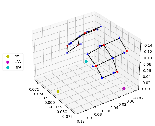
cedalion.vis.anatomy.plot_montage3D(data["sub-01"]["amp"], data["sub-01"].geo3d, landmarks=["Nz", "Iz", "LPA", "RPA", "Cz"])
Plot preprocessed data
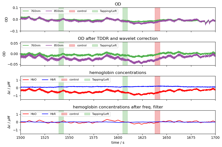
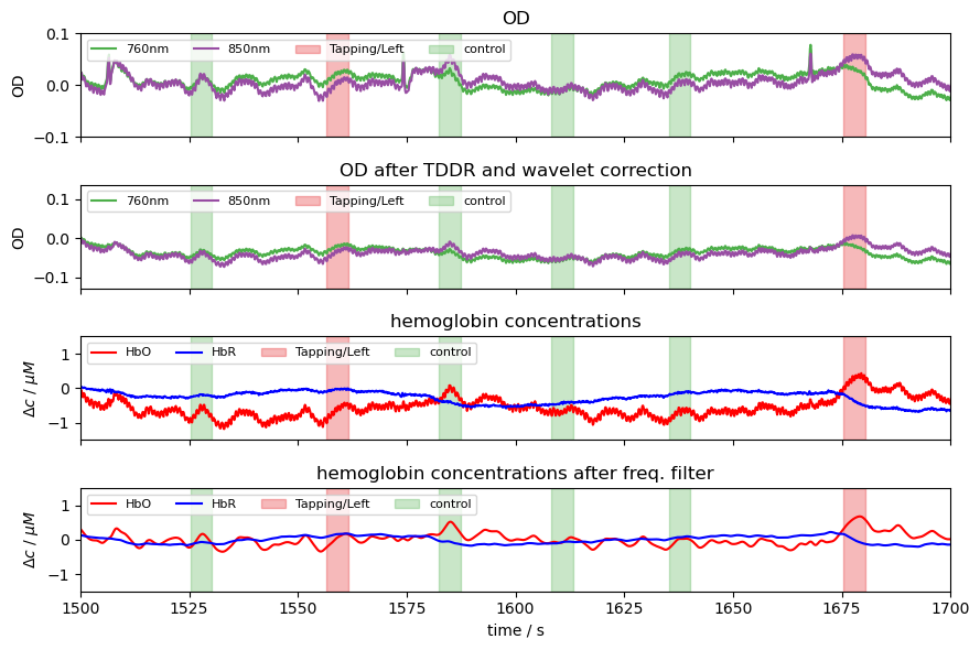
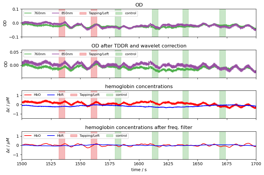
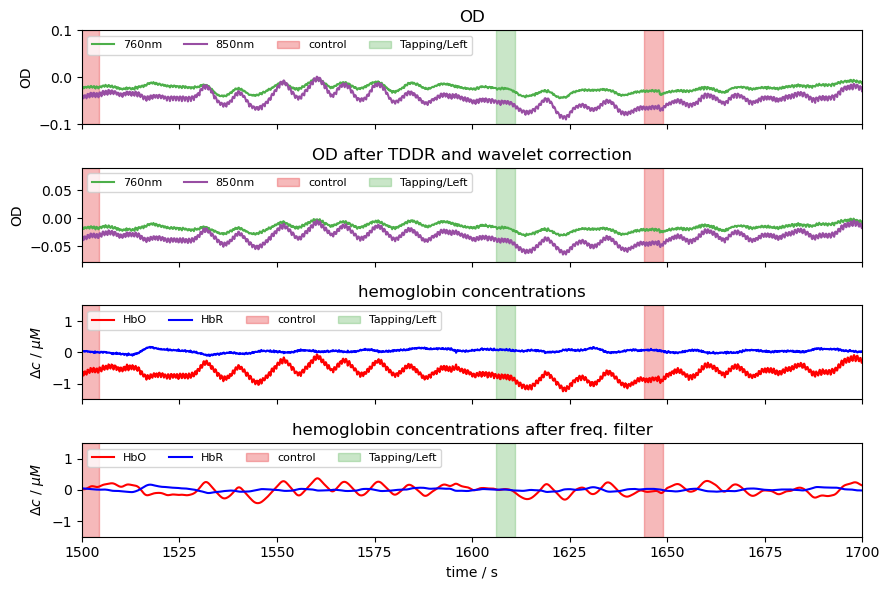
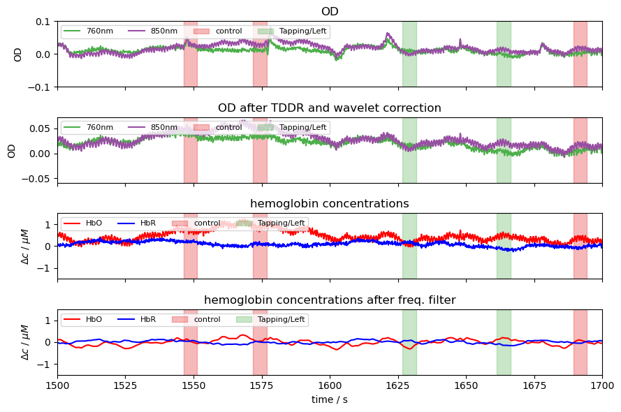
Illustrate for a single subject and channel the effect of the preprocessing.
[6]:
for i_sub, subject in enumerate(subjects):

    rec = data[subject]
    channel = "S2D4"
    od_ylims = (-.1,.1)
    conc_ylims = (-1.5,1.5)

    f, ax = p.subplots(4, 1, figsize=(9, 6), sharex=True)


    ax[0].plot(rec["od"].time, rec["od"].sel(channel=channel, wavelength=760), c="#4daf4a", label="760nm")
    ax[0].plot(rec["od"].time, rec["od"].sel(channel=channel, wavelength=850), c="#984ea3", label="850nm")
    ax[0].set_ylabel("OD")
    ax[0].set_title("OD")
    ax[0].set_ylim(*od_ylims)

    ax[1].plot(rec["od_wavelet"].time, rec["od_wavelet"].sel(channel=channel, wavelength=760), c="#4daf4a", label="760nm")
    ax[1].plot(rec["od_wavelet"].time, rec["od_wavelet"].sel(channel=channel, wavelength=850), c="#984ea3", label="850nm")
    ax[1].set_ylabel("OD")
    ax[1].set_title("OD after TDDR and wavelet correction")
    ax[0].set_ylim(*od_ylims)

    ax[2].plot(rec["conc"].time, rec["conc"].sel(channel=channel, chromo="HbO"), "r-", label="HbO")
    ax[2].plot(rec["conc"].time, rec["conc"].sel(channel=channel, chromo="HbR"), "b-", label="HbR")
    ax[2].set_ylabel("$\Delta c$ / $\mu M$")
    ax[2].set_title("hemoglobin concentrations")
    ax[2].set_ylim(*conc_ylims)

    ax[3].plot(rec["conc_freqfilt"].time, rec["conc_freqfilt"].sel(channel=channel, chromo="HbO"), "r-", label="HbO")
    ax[3].plot(rec["conc_freqfilt"].time, rec["conc_freqfilt"].sel(channel=channel, chromo="HbR"), "b-", label="HbR")
    ax[3].set_ylabel("$\Delta c$ / $\mu M$")
    ax[3].set_title("hemoglobin concentrations after freq. filter")
    ax[3].set_ylim(*conc_ylims)

    ax[0].set_xlim(1500, 1700)
    ax[3].set_xlabel("time / s")

    for a in ax:
        cedalion.vis.blocks.plot_stim_markers(a, rec.stim, y=1.)
        a.legend(loc="upper left", ncol=5, fontsize=8)
    f.tight_layout()
Show channel quality per subject
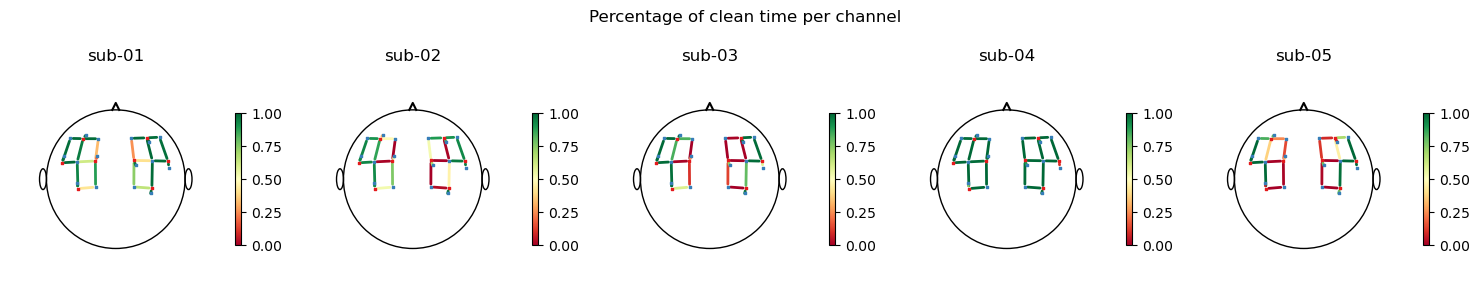
Create for each subject a scalp plot which shows for each channel the fraction of time windows in which the data quality is considered good. The preprocessing pruned channels which are bad more than 50% of the time.
[7]:
f, ax = p.subplots(1, 5, figsize=(15, 3))
for i, sub in enumerate(subjects):
    rec = data[sub]

    cedalion.vis.anatomy.scalp_plot(
        rec["od"],
        rec.geo3d,
        rec.aux_obj["perc_time_clean"],
        ax=ax[i],
        optode_size=2,
        title=sub,
        cmap="RdYlGn",
        vmin=0.0,
        vmax=1,
    )

f.suptitle("Percentage of clean time per channel")
f.tight_layout()
Short-channel regression and epoching
Using the GLM in single-trial analysis requires careful handling of the design matrix and regression step to avoid data leakage. The simple implementation below follows the recipe outlined in [vLOMBY20], see the paper for more details.
Define a function that, for a single subject:
splits the trials into 4 cross-validation folds
defines a GLM design matrix with HRF and short-channel regressors
blanks the design matrix during the test trials of each cv. fold
fits the GLM and subtracts the component explained by the short-channel regressor
splits the SSC-corrected time series into epochs
subtracts a baseline from each epoch
returns a list of arrays, one per cv fold; each array contains all epochs with coordinates attached that allow train and test trials to be distinguished
[8]:
def process_single_subject(rec, subtract_global_component: bool) -> list[xr.DataArray]:

    n_splits = 4
    before = 2 * cedalion.units.s
    after = 15 * cedalion.units.s

    cv_folds = []

    # separate long and short channels
    rec["conc_long"], rec["conc_short"] = cedalion.nirs.split_long_short_channels(
        rec["conc_freqfilt"], rec.geo3d, distance_threshold=15.0 * units.mm
    )

    # split trials into train and test for n_splits CV folds
    for i_split, (df_stim_train, df_stim_test) in enumerate(
        mlutils.cv.create_cv_splits(rec.stim, n_splits)
    ):
        if subtract_global_component:
            # define the GLM design matrix
            dms = glm.design_matrix.hrf_regressors(
                rec["conc_long"],
                rec.stim,
                glm.Gamma(tau=0 * units.s, sigma=3 * units.s),
            ) & glm.design_matrix.average_short_channel_regressor(rec["conc_short"])

            # zero-out design matrix in test segment
            dms_masked = mlutils.cv.mask_design_matrix(
                dms,
                df_stim_test,
                before=before,
                after=after,
            )

            # fit long channels with masked design matrix
            result = glm.fit(rec["conc_long"], dms_masked, noise_model="ols")

            # compute component explained by short-channel regressor
            short_component = glm.predict(
                rec["conc_long"],
                result.sm.params.sel(regressor=["short"]),
                dms,
            )
            short_component = short_component.pint.quantify(rec["conc_long"].pint.units)

            # subtract short component
            conc_for_epoching = rec["conc_long"] - short_component
        else:
            conc_for_epoching = rec["conc_long"]

        # split time series into epochs
        epochs = conc_for_epoching.cd.to_epochs(
            rec.stim,
            # ["Tapping/Left", "Tapping/Right"],
            ["control", "Tapping/Left"],
            before=before,
            after=after,
        )

        # baseline correction
        baseline = epochs.sel(reltime=(epochs.reltime < 0)).mean("reltime")
        epochs = epochs - baseline

        # assign train-/test-set membership...
        is_train = np.zeros(epochs.sizes["epoch"], dtype=bool)
        is_test = np.zeros(epochs.sizes["epoch"], dtype=bool)
        is_train[df_stim_train.index.values] = True
        is_test[df_stim_test.index.values] = True

        # ... and digitized trial labels ...
        # (0,1,.. instead of "Tapping/Left", "Tapping/Right"...)
        label_encoder = LabelEncoder()
        y = label_encoder.fit_transform(epochs.trial_type.values)

        # ... as coordinates to the DataArray
        epochs = epochs.assign_coords(
            {
                "is_train": ("epoch", is_train),
                "is_test": ("epoch", is_test),
                "y": ("epoch", y),
            }
        )

        cv_folds.append(epochs)

    return cv_folds
Inspect the arrays representing a CV fold. These are epoched time series with one epoch per trial arranged along dimension 'epoch'. The coordinates is_train, is_test describe for each epoch if it is part of the train of test set. The different folds contain the same epochs with different assignments of trials to the train/test sets. The coordinate y is a numeric representation of the trial_type as required by scikit-learn classifiers.
[9]:
cv_folds = process_single_subject(data["sub-01"], subtract_global_component=False)

display(cv_folds[0])
display(cv_folds[-1])
<xarray.DataArray (epoch: 60, chromo: 2, channel: 16, reltime: 135)> Size: 2MB
<Quantity([[[[-9.3714e-02 -7.8124e-02 -6.2774e-02 ... -8.6741e-02 -9.7942e-02
    -1.0924e-01]
   [-9.5185e-02 -8.5083e-02 -7.4190e-02 ... -1.6120e-01 -1.5882e-01
    -1.5665e-01]
   [-7.1943e-02 -5.9558e-02 -4.7282e-02 ... -1.8900e-01 -1.9434e-01
    -2.0007e-01]
   ...
   [-1.2025e-01 -1.0697e-01 -9.2745e-02 ... -4.4288e-01 -4.5381e-01
    -4.6637e-01]
   [-8.7524e-02 -7.4605e-02 -6.1478e-02 ... -3.9973e-01 -4.0392e-01
    -4.0840e-01]
   [-5.8143e-02 -4.9710e-02 -4.0982e-02 ... -3.9304e-01 -3.9282e-01
    -3.9267e-01]]

  [[ 2.4046e-03  1.2129e-03  3.2792e-04 ... -6.0494e-02 -4.9949e-02
    -4.0034e-02]
   [ 8.1752e-03  1.0916e-02  1.2657e-02 ... -2.3302e-02 -2.7449e-02
    -3.2918e-02]
   [ 5.3153e-03  1.9881e-03 -9.6345e-04 ... -5.5447e-02 -5.1820e-02
    -4.8051e-02]
...
   [ 8.6953e-02  7.6663e-02  6.5407e-02 ...  2.3010e-02  3.8361e-02
     5.3422e-02]
   [ 7.3274e-02  6.5880e-02  5.7208e-02 ...  1.0535e-01  1.1702e-01
     1.2830e-01]
   [ 3.2520e-02  2.6869e-02  2.0952e-02 ...  3.5230e-01  3.6504e-01
     3.7687e-01]]

  [[-1.9129e-02 -1.5943e-02 -1.2350e-02 ...  5.0320e-02  5.0038e-02
     4.8112e-02]
   [-2.4353e-02 -2.3238e-02 -1.9715e-02 ...  2.3422e-02  2.2695e-02
     2.0638e-02]
   [-1.2239e-02 -1.3154e-02 -1.3375e-02 ...  6.7565e-02  6.8972e-02
     7.0489e-02]
   ...
   [ 9.5585e-04 -2.4874e-03 -6.2408e-03 ...  9.1244e-02  9.4591e-02
     9.8010e-02]
   [-1.0578e-02 -1.1294e-02 -1.1444e-02 ...  4.6553e-03  5.6745e-03
     6.5657e-03]
   [ 5.7040e-03  4.0702e-03  1.8860e-03 ... -2.2583e-02 -2.1053e-02
    -1.9265e-02]]]], 'micromolar')>
Coordinates: (3/9)
  * reltime     (reltime) float64 1kB -2.048 -1.92 -1.792 ... 14.85 14.98 15.1
    trial_type  (epoch) <U12 3kB 'control' 'control' ... 'Tapping/Left'
    ...          ...
    y           (epoch) int64 480B 1 1 1 0 0 1 0 0 0 0 1 ... 1 0 0 1 1 0 1 0 1 0
Dimensions without coordinates: epoch<xarray.DataArray (epoch: 60, chromo: 2, channel: 16, reltime: 135)> Size: 2MB
<Quantity([[[[-9.3714e-02 -7.8124e-02 -6.2774e-02 ... -8.6741e-02 -9.7942e-02
-1.0924e-01]
[-9.5185e-02 -8.5083e-02 -7.4190e-02 ... -1.6120e-01 -1.5882e-01
-1.5665e-01]
[-7.1943e-02 -5.9558e-02 -4.7282e-02 ... -1.8900e-01 -1.9434e-01
-2.0007e-01]
...
[-1.2025e-01 -1.0697e-01 -9.2745e-02 ... -4.4288e-01 -4.5381e-01
-4.6637e-01]
[-8.7524e-02 -7.4605e-02 -6.1478e-02 ... -3.9973e-01 -4.0392e-01
-4.0840e-01]
[-5.8143e-02 -4.9710e-02 -4.0982e-02 ... -3.9304e-01 -3.9282e-01
-3.9267e-01]]
[[ 2.4046e-03 1.2129e-03 3.2792e-04 ... -6.0494e-02 -4.9949e-02
-4.0034e-02]
[ 8.1752e-03 1.0916e-02 1.2657e-02 ... -2.3302e-02 -2.7449e-02
-3.2918e-02]
[ 5.3153e-03 1.9881e-03 -9.6345e-04 ... -5.5447e-02 -5.1820e-02
-4.8051e-02]
...
[ 8.6953e-02 7.6663e-02 6.5407e-02 ... 2.3010e-02 3.8361e-02
5.3422e-02]
[ 7.3274e-02 6.5880e-02 5.7208e-02 ... 1.0535e-01 1.1702e-01
1.2830e-01]
[ 3.2520e-02 2.6869e-02 2.0952e-02 ... 3.5230e-01 3.6504e-01
3.7687e-01]]
[[-1.9129e-02 -1.5943e-02 -1.2350e-02 ... 5.0320e-02 5.0038e-02
4.8112e-02]
[-2.4353e-02 -2.3238e-02 -1.9715e-02 ... 2.3422e-02 2.2695e-02
2.0638e-02]
[-1.2239e-02 -1.3154e-02 -1.3375e-02 ... 6.7565e-02 6.8972e-02
7.0489e-02]
...
[ 9.5585e-04 -2.4874e-03 -6.2408e-03 ... 9.1244e-02 9.4591e-02
9.8010e-02]
[-1.0578e-02 -1.1294e-02 -1.1444e-02 ... 4.6553e-03 5.6745e-03
6.5657e-03]
[ 5.7040e-03 4.0702e-03 1.8860e-03 ... -2.2583e-02 -2.1053e-02
-1.9265e-02]]]], 'micromolar')>
Coordinates: (3/9)
* reltime (reltime) float64 1kB -2.048 -1.92 -1.792 ... 14.85 14.98 15.1
trial_type (epoch) <U12 3kB 'control' 'control' ... 'Tapping/Left'
... ...
y (epoch) int64 480B 1 1 1 0 0 1 0 0 0 0 1 ... 1 0 0 1 1 0 1 0 1 0
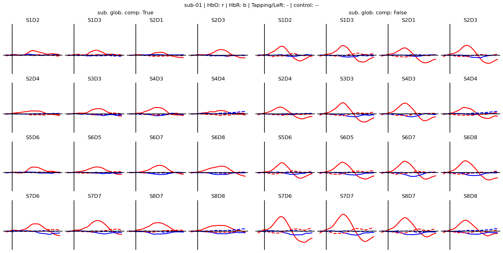
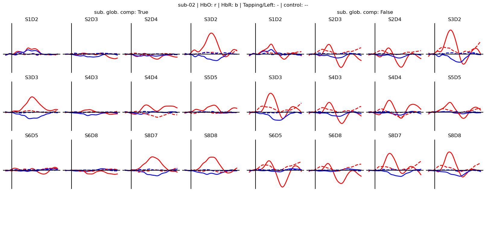
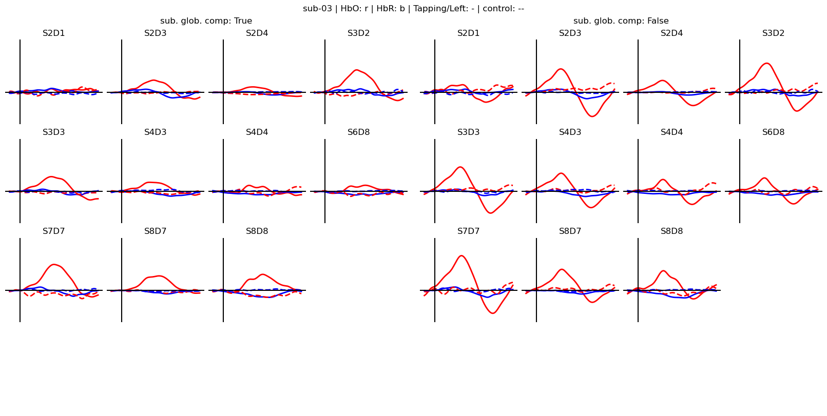
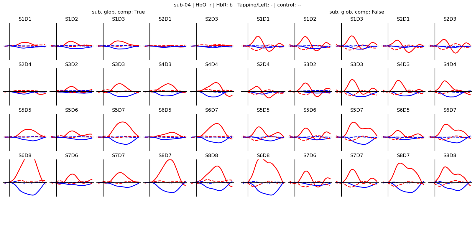
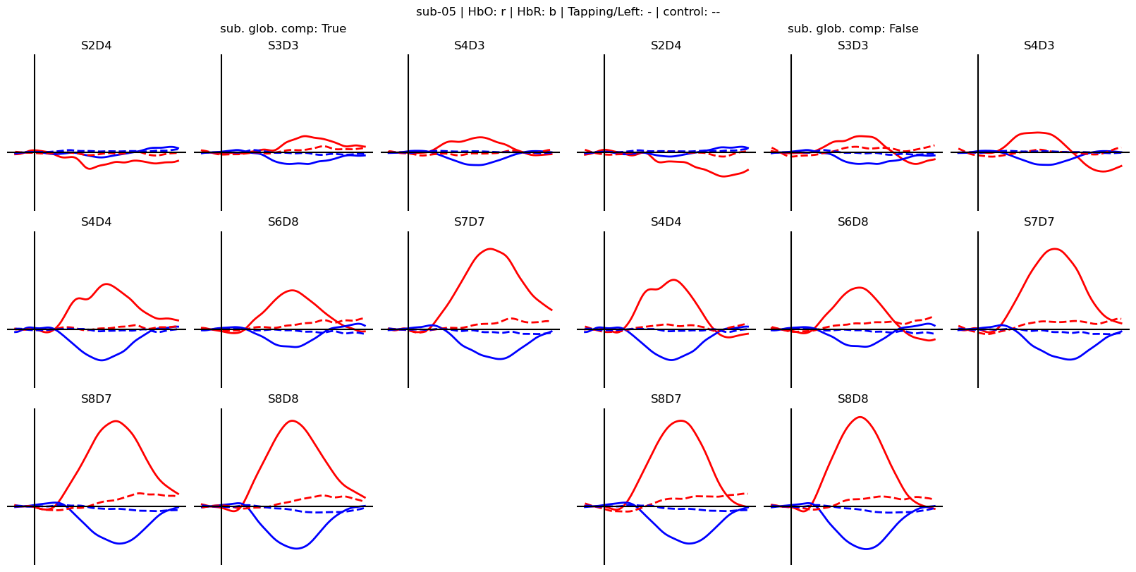
Dimensions without coordinates: epochInspect the effect of global-component subtraction. Run process_single_subject for each subject with and without global-component subtraction. Then group and average epochs per trial type (block average) to estimate the hemodynamic response function in each channel.
[10]:
for sub in subjects:

    f = p.figure(figsize=(16, 8), constrained_layout=True)
    subfigs = f.subfigures(1, 2)

    for subfig, subtract_global_component in zip(subfigs, [True, False]):

        cv_folds = cv_folds = process_single_subject(data[sub], subtract_global_component)

        blockaverage = cv_folds[0].groupby("trial_type").mean("epoch")

        # Plot block averages. Please ignore errors if the plot is too small in the HD case

        noPlts2 = int(np.ceil(np.sqrt(len(blockaverage.channel))))

        ax = subfig.subplots(noPlts2, noPlts2).flatten()

        for i_ch, ch in enumerate(blockaverage.channel):
            for ls, trial_type in zip(["-", "--"], blockaverage.trial_type):
                ax[i_ch].plot(blockaverage.reltime, blockaverage.sel(chromo="HbO", trial_type=trial_type, channel=ch), "r", lw=2, ls=ls)
                ax[i_ch].plot(blockaverage.reltime, blockaverage.sel(chromo="HbR", trial_type=trial_type, channel=ch), "b", lw=2, ls=ls)

            ax[i_ch].grid(1)
            ax[i_ch].set_title(ch.values)
            ax[i_ch].set_ylim(-.3, .5)
            ax[i_ch].set_axis_off()
            ax[i_ch].axhline(0, c="k")
            ax[i_ch].axvline(0, c="k")

        for i in range(len(blockaverage.channel), len(ax)):
            ax[i].set_axis_off()

        subfig.suptitle(f"sub. glob. comp: {subtract_global_component}")
        #subfig.suptitle(f"HbO: r | HbR: b | left: - | right: -- | sub. glob. comp: {subtract_global_component}")

    f.suptitle(f"{sub} | HbO: r | HbR: b | {blockaverage.trial_type.values[0]}: - | {blockaverage.trial_type.values[1]}: --")
 94%|█████████▍| 15/16 [00:00<00:00, 356.18it/s]
 94%|█████████▍| 15/16 [00:00<00:00, 290.25it/s]
 94%|█████████▍| 15/16 [00:00<00:00, 303.61it/s]
 94%|█████████▍| 15/16 [00:00<00:00, 293.94it/s]
 94%|█████████▍| 15/16 [00:00<00:00, 285.40it/s]
 94%|█████████▍| 15/16 [00:00<00:00, 388.71it/s]
 94%|█████████▍| 15/16 [00:00<00:00, 301.78it/s]
 94%|█████████▍| 15/16 [00:00<00:00, 300.70it/s]
 92%|█████████▏| 11/12 [00:00<00:00, 400.76it/s]
 92%|█████████▏| 11/12 [00:00<00:00, 417.58it/s]
 92%|█████████▏| 11/12 [00:00<00:00, 385.27it/s]
 92%|█████████▏| 11/12 [00:00<00:00, 304.62it/s]
 92%|█████████▏| 11/12 [00:00<00:00, 287.14it/s]
 92%|█████████▏| 11/12 [00:00<00:00, 403.48it/s]
 92%|█████████▏| 11/12 [00:00<00:00, 422.54it/s]
 92%|█████████▏| 11/12 [00:00<00:00, 444.16it/s]
 91%|█████████ | 10/11 [00:00<00:00, 162.16it/s]
 91%|█████████ | 10/11 [00:00<00:00, 179.46it/s]
 91%|█████████ | 10/11 [00:00<00:00, 127.66it/s]
 91%|█████████ | 10/11 [00:00<00:00, 158.48it/s]
 91%|█████████ | 10/11 [00:00<00:00, 191.95it/s]
 91%|█████████ | 10/11 [00:00<00:00, 259.08it/s]
 91%|█████████ | 10/11 [00:00<00:00, 196.43it/s]
 91%|█████████ | 10/11 [00:00<00:00, 374.86it/s]
 95%|█████████▌| 19/20 [00:00<00:00, 363.10it/s]
 95%|█████████▌| 19/20 [00:00<00:00, 342.19it/s]
 95%|█████████▌| 19/20 [00:00<00:00, 341.92it/s]
 95%|█████████▌| 19/20 [00:00<00:00, 371.19it/s]
 95%|█████████▌| 19/20 [00:00<00:00, 366.56it/s]
 95%|█████████▌| 19/20 [00:00<00:00, 356.33it/s]
 95%|█████████▌| 19/20 [00:00<00:00, 298.78it/s]
 95%|█████████▌| 19/20 [00:00<00:00, 358.33it/s]
 88%|████████▊ | 7/8 [00:00<00:00, 288.39it/s]
 88%|████████▊ | 7/8 [00:00<00:00, 284.64it/s]
 88%|████████▊ | 7/8 [00:00<00:00, 298.08it/s]
 88%|████████▊ | 7/8 [00:00<00:00, 293.19it/s]
 88%|████████▊ | 7/8 [00:00<00:00, 261.64it/s]
 88%|████████▊ | 7/8 [00:00<00:00, 277.93it/s]
 88%|████████▊ | 7/8 [00:00<00:00, 280.06it/s]
 88%|████████▊ | 7/8 [00:00<00:00, 258.41it/s]
The function mlutils.features.epoch_features calculates common features of the hemodynamic response, such as slope, mean, maximum, minimum and area under the curve. For each feature type, a time range can be specified over which the feature is calculated. In the present case, this yields features for each channel and chromophore, which are then stacked into a single feature dimension. The resulting array has the shape expected by scikit-learn, (\(N_{samples}\), \(N_{features}\)).
[11]:
X = mlutils.features.epoch_features(
    cv_folds[0],
    feature_types=["slope", "mean", "max", "min", "auc"],
    reltime_slices={
        "slope": slice(0, 9),
        "mean": slice(3, 10),
        "max": slice(2, 8),
        "min": slice(2, 8),
    },
)
X
[11]:
<xarray.DataArray (epoch: 60, feature: 80)> Size: 38kB
array([[ 0.0075,  0.0044,  0.0057, ...,  0.2717,  0.2893,  0.3286],
       [ 0.0393,  0.0229,  0.0067, ..., -0.2663, -1.2641, -0.6725],
       [-0.0049,  0.0025, -0.0078, ..., -0.6788,  1.1415, -0.188 ],
       ...,
       [ 0.0473,  0.0486,  0.0491, ...,  1.2899,  0.0246, -0.2599],
       [ 0.0082, -0.0168, -0.0023, ...,  0.1861, -0.8478, -0.8331],
       [-0.0158,  0.025 ,  0.0033, ..., -2.2424, -1.7198, -2.0566]],
      shape=(60, 80))
Coordinates: (3/10)
    trial_type    (epoch) <U12 3kB 'control' 'control' ... 'Tapping/Left'
    source        (feature) object 640B 'S2' 'S3' 'S4' 'S4' ... 'S7' 'S8' 'S8'
    ...            ...
  * channel       (feature) object 640B 'S2D4' 'S3D3' 'S4D3' ... 'S8D7' 'S8D8'
Dimensions without coordinates: epochClassifciation with and without short-channel regression
Process each subject, extract features and train a LDA classifier, calculate classification accuracies.
[12]:
accuracies = defaultdict(list)


for sub in subjects:
    for subtract_global_component in [True, False]:
        key = (sub, subtract_global_component)

        rec = data[sub]
        cv_folds = process_single_subject(rec, subtract_global_component)

        for epochs in cv_folds:
            # extract features
            X = mlutils.features.epoch_features(
                epochs.sel(chromo="HbO"),  # HbO only
                feature_types=["slope", "max", "mean"],
                reltime_slices={
                    "slope": slice(0, 9),
                    # "auc" : slice(0, 9),
                    "mean": slice(3, 10),
                    "max": slice(2, 8),
                },
            )

            # separate train and test sets
            X_train = X[X.is_train]
            y_train = X_train.y
            X_test = X[X.is_test]
            y_test = X_test.y

            # train a LDA classifier

            clf = make_pipeline(
                StandardScaler(),
                LinearDiscriminantAnalysis(
                    n_components=1, solver="lsqr", shrinkage="auto"
                ),
            )
            # clf = LinearDiscriminantAnalysis(n_components=1, solver='lsqr', shrinkage="auto")
            clf.fit(X_train, y_train)

            # evaluate perfomance
            accuracy = clf.score(X_test, y_test)

            accuracies[key].append(accuracy)
            print(
                f"{sub} - #train: {len(y_train)} #test: {len(y_test)} #features: {X_train.shape[1]} accuracy: {accuracy:.3f}"
            )

        print(
            rf"{sub} subtract global: {subtract_global_component} - average accuracy over cross-validation splits: {np.mean(accuracies[key]):.3f} ± {np.std(accuracies[key]):.3f}"
        )
        print("-" * 80)
 94%|█████████▍| 15/16 [00:00<00:00, 253.99it/s]
 94%|█████████▍| 15/16 [00:00<00:00, 169.25it/s]
 94%|█████████▍| 15/16 [00:00<00:00, 296.50it/s]
 94%|█████████▍| 15/16 [00:00<00:00, 268.30it/s]
 94%|█████████▍| 15/16 [00:00<00:00, 175.81it/s]
 94%|█████████▍| 15/16 [00:00<00:00, 218.82it/s]
 94%|█████████▍| 15/16 [00:00<00:00, 236.82it/s]
 94%|█████████▍| 15/16 [00:00<00:00, 360.34it/s]
sub-01 - #train: 45 #test: 15 #features: 48 accuracy: 0.867
sub-01 - #train: 45 #test: 15 #features: 48 accuracy: 0.800
sub-01 - #train: 45 #test: 15 #features: 48 accuracy: 0.733
sub-01 - #train: 45 #test: 15 #features: 48 accuracy: 0.867
sub-01 subtract global: True - average accuracy over cross-validation splits: 0.817 ± 0.055
--------------------------------------------------------------------------------
sub-01 - #train: 45 #test: 15 #features: 48 accuracy: 0.800
sub-01 - #train: 45 #test: 15 #features: 48 accuracy: 0.733
sub-01 - #train: 45 #test: 15 #features: 48 accuracy: 0.667
sub-01 - #train: 45 #test: 15 #features: 48 accuracy: 0.800
sub-01 subtract global: False - average accuracy over cross-validation splits: 0.750 ± 0.055
--------------------------------------------------------------------------------
 92%|█████████▏| 11/12 [00:00<00:00, 263.66it/s]
 92%|█████████▏| 11/12 [00:00<00:00, 301.55it/s]
 92%|█████████▏| 11/12 [00:00<00:00, 259.21it/s]
 92%|█████████▏| 11/12 [00:00<00:00, 278.72it/s]
 92%|█████████▏| 11/12 [00:00<00:00, 369.02it/s]
 92%|█████████▏| 11/12 [00:00<00:00, 203.33it/s]
 92%|█████████▏| 11/12 [00:00<00:00, 157.41it/s]
 92%|█████████▏| 11/12 [00:00<00:00, 170.62it/s]
sub-02 - #train: 45 #test: 15 #features: 36 accuracy: 0.933
sub-02 - #train: 45 #test: 15 #features: 36 accuracy: 0.800
sub-02 - #train: 45 #test: 15 #features: 36 accuracy: 0.933
sub-02 - #train: 45 #test: 15 #features: 36 accuracy: 0.800
sub-02 subtract global: True - average accuracy over cross-validation splits: 0.867 ± 0.067
--------------------------------------------------------------------------------
sub-02 - #train: 45 #test: 15 #features: 36 accuracy: 0.867
sub-02 - #train: 45 #test: 15 #features: 36 accuracy: 0.800
sub-02 - #train: 45 #test: 15 #features: 36 accuracy: 0.800
sub-02 - #train: 45 #test: 15 #features: 36 accuracy: 0.867
sub-02 subtract global: False - average accuracy over cross-validation splits: 0.833 ± 0.033
--------------------------------------------------------------------------------
 91%|█████████ | 10/11 [00:00<00:00, 376.71it/s]
 91%|█████████ | 10/11 [00:00<00:00, 252.70it/s]
 91%|█████████ | 10/11 [00:00<00:00, 248.53it/s]
 91%|█████████ | 10/11 [00:00<00:00, 265.45it/s]
 91%|█████████ | 10/11 [00:00<00:00, 256.82it/s]
 91%|█████████ | 10/11 [00:00<00:00, 166.23it/s]
 91%|█████████ | 10/11 [00:00<00:00, 281.93it/s]
 91%|█████████ | 10/11 [00:00<00:00, 259.09it/s]
sub-03 - #train: 45 #test: 15 #features: 33 accuracy: 0.933
sub-03 - #train: 45 #test: 15 #features: 33 accuracy: 0.733
sub-03 - #train: 45 #test: 15 #features: 33 accuracy: 0.733
sub-03 - #train: 45 #test: 15 #features: 33 accuracy: 0.933
sub-03 subtract global: True - average accuracy over cross-validation splits: 0.833 ± 0.100
--------------------------------------------------------------------------------
sub-03 - #train: 45 #test: 15 #features: 33 accuracy: 0.800
sub-03 - #train: 45 #test: 15 #features: 33 accuracy: 0.800
sub-03 - #train: 45 #test: 15 #features: 33 accuracy: 0.733
sub-03 - #train: 45 #test: 15 #features: 33 accuracy: 0.800
sub-03 subtract global: False - average accuracy over cross-validation splits: 0.783 ± 0.029
--------------------------------------------------------------------------------
 95%|█████████▌| 19/20 [00:00<00:00, 188.09it/s]
 95%|█████████▌| 19/20 [00:00<00:00, 166.21it/s]
 95%|█████████▌| 19/20 [00:00<00:00, 234.00it/s]
 95%|█████████▌| 19/20 [00:00<00:00, 288.37it/s]
 95%|█████████▌| 19/20 [00:00<00:00, 192.21it/s]
 95%|█████████▌| 19/20 [00:00<00:00, 220.31it/s]
 95%|█████████▌| 19/20 [00:00<00:00, 250.02it/s]
 95%|█████████▌| 19/20 [00:00<00:00, 329.68it/s]
sub-04 - #train: 45 #test: 15 #features: 60 accuracy: 0.933
sub-04 - #train: 45 #test: 15 #features: 60 accuracy: 1.000
sub-04 - #train: 45 #test: 15 #features: 60 accuracy: 0.867
sub-04 - #train: 45 #test: 15 #features: 60 accuracy: 1.000
sub-04 subtract global: True - average accuracy over cross-validation splits: 0.950 ± 0.055
--------------------------------------------------------------------------------
sub-04 - #train: 45 #test: 15 #features: 60 accuracy: 1.000
sub-04 - #train: 45 #test: 15 #features: 60 accuracy: 1.000
sub-04 - #train: 45 #test: 15 #features: 60 accuracy: 0.933
sub-04 - #train: 45 #test: 15 #features: 60 accuracy: 1.000
sub-04 subtract global: False - average accuracy over cross-validation splits: 0.983 ± 0.029
--------------------------------------------------------------------------------
 88%|████████▊ | 7/8 [00:00<00:00, 192.59it/s]
 88%|████████▊ | 7/8 [00:00<00:00, 253.73it/s]
 88%|████████▊ | 7/8 [00:00<00:00, 205.61it/s]
 88%|████████▊ | 7/8 [00:00<00:00, 438.44it/s]
 88%|████████▊ | 7/8 [00:00<00:00, 260.90it/s]
 88%|████████▊ | 7/8 [00:00<00:00, 190.05it/s]
 88%|████████▊ | 7/8 [00:00<00:00, 194.78it/s]
 88%|████████▊ | 7/8 [00:00<00:00, 268.57it/s]
sub-05 - #train: 45 #test: 15 #features: 24 accuracy: 1.000
sub-05 - #train: 45 #test: 15 #features: 24 accuracy: 0.933
sub-05 - #train: 45 #test: 15 #features: 24 accuracy: 0.933
sub-05 - #train: 45 #test: 15 #features: 24 accuracy: 1.000
sub-05 subtract global: True - average accuracy over cross-validation splits: 0.967 ± 0.033
--------------------------------------------------------------------------------
sub-05 - #train: 45 #test: 15 #features: 24 accuracy: 0.933
sub-05 - #train: 45 #test: 15 #features: 24 accuracy: 0.867
sub-05 - #train: 45 #test: 15 #features: 24 accuracy: 0.933
sub-05 - #train: 45 #test: 15 #features: 24 accuracy: 0.933
sub-05 subtract global: False - average accuracy over cross-validation splits: 0.917 ± 0.029
--------------------------------------------------------------------------------
Calculate confidence intervals for measured accuracies and compare the performance with and without short-channel regression.
[13]:
from statsmodels.stats.proportion import proportion_confint


def acc_and_ci(fold_accs, n_per_fold=15):
    """Pooled accuracy and Wilson-CI error-bar lengths (lower, upper)."""
    n_total = n_per_fold * len(fold_accs)
    n_correct = round(sum(fold_accs) * n_per_fold)
    mean = n_correct / n_total
    lo, hi = proportion_confint(n_correct, n_total, alpha=0.05, method="wilson")
    return mean, mean - lo, hi - mean

f, ax = p.subplots(figsize=(8, 6))
x = np.arange(len(subjects))

for dx, use_scc, fmt, label in [(-.1, False, "rs", "No SS correction"),
                                (+.1, True,  "gs", "SS correction")]:
    mean, lo, hi = np.array([acc_and_ci(accuracies[s, use_scc]) for s in subjects]).T
    ax.errorbar(x + dx, mean, yerr=[lo, hi], fmt=fmt, label=label)

ax.set_xticks(x)
ax.set_xticklabels(subjects)
ax.axhline(0.5, c="k", ls="--", label="chance")
ax.legend(loc="center right")
ax.set_ylim(0.45, 1.05)
ax.set_ylabel("accuracy")
[13]:
Text(0, 0.5, 'accuracy')
Bonus: classification in image (parcel) space
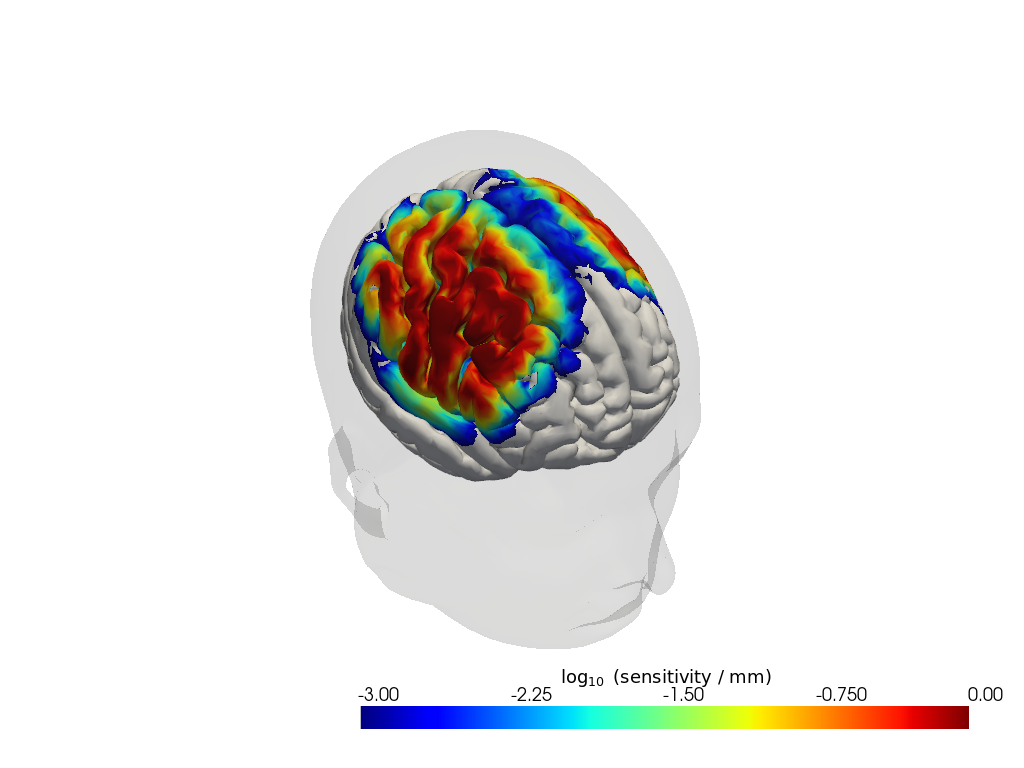
So far, all classification was done on channel-space concentration data, where each feature is tied to a specific source-detector pair. Cedalion can also solve the DOT inverse problem to project channel-space data onto the cortical surface (“image reconstruction”), which yields a representation that is independent of the particular probe geometry and can be interpreted anatomically.
Caveat: the probe used in this dataset is a comparatively sparse, single- distance montage covering only motor cortex — far from the high-density layouts for which DOT image reconstruction is designed and validated. Image reconstruction from such a sparse probe is inherently ill-posed and cannot recover the same spatial detail or SNR that a dense array would provide. We reconstruct images here anyway, not because it is the ideal use case, but to demonstrate how to go from channel-space data to parcel-space features and classify on them with cedalion — the same workflow applies directly to higher-density probes, where image-space classification is expected to be more advantageous (see the note on [FMMvonLuhmann26] above).
In this section we:
Load a precomputed sensitivity (Adot) matrix for this probe montage (
cedalion.data.get_precomputed_sensitivity). This is the linear forward operator that maps absorption changes at every vertex of the cortical surface to optical density changes at every channel/wavelength.Build an
cedalion.dot.ImageReconobject that solves the (regularized) inverse problem, and use it to reconstruct HbO/HbR concentration images directly from optical density.Determine which cortical parcels (Schaefer2018 atlas) this probe is actually sensitive to, using
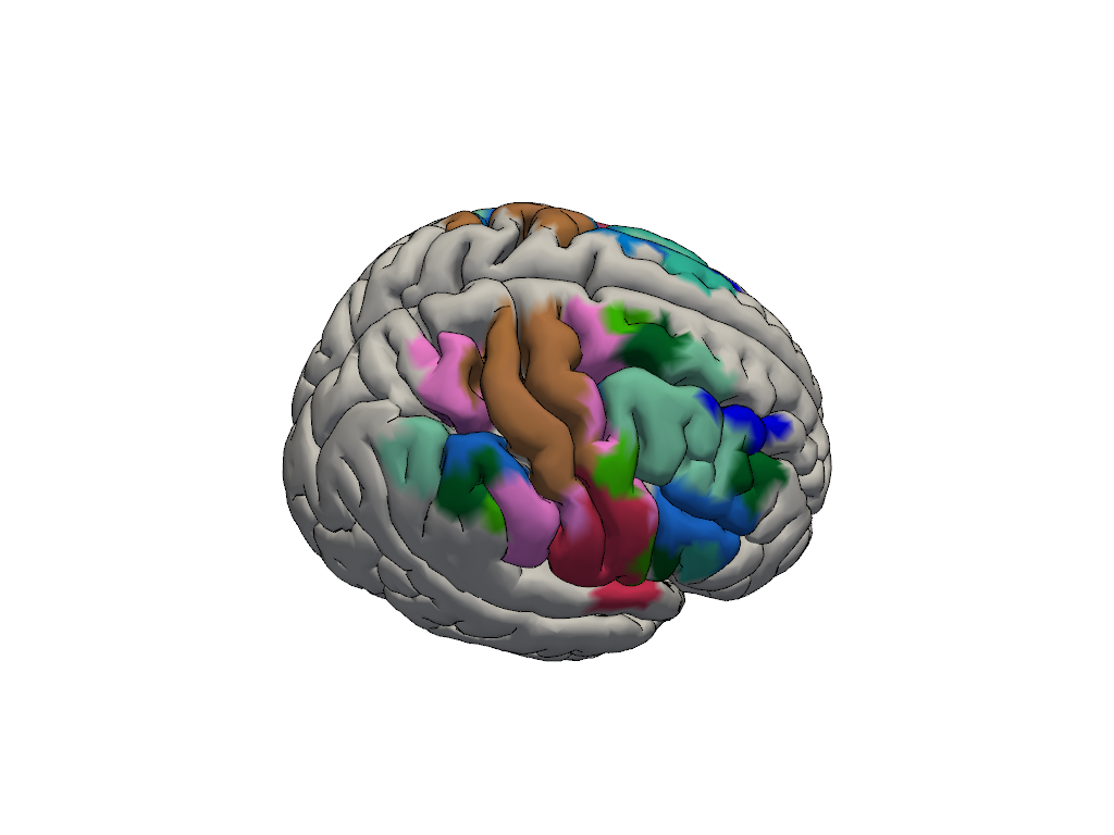
ForwardModel.parcel_sensitivity, and restrict the analysis to those parcels only — regions the montage cannot see should not be used as classifier features.Reconstruct images from
od_wavelet— the optical density time series right after TDDR and wavelet motion correction (the same starting point used for the channel-spaceSS correction: Falsecondition above), i.e. without any short-channel/GLM regression — and average vertex-space images into brain parcels.Extract the same slope/mean/max features used for channel-space classification, this time per parcel instead of per channel, and train and cross-validate the same LDA pipeline.
Compare parcel-space accuracy to the channel-space accuracy obtained above (
No SS correctioncondition), since both use the same preprocessing stage and no short-channel regression.
[14]:
HEAD_MODEL = "icbm152"

# precomputed sensitivity (Adot) matrix for this probe montage, on the
# standard icbm152 head model. dims: (channel, vertex, wavelength);
# vertex coords include "is_brain" and "parcel" (Schaefer2018 atlas label).
Adot = cedalion.data.get_precomputed_sensitivity("fingertapping", HEAD_MODEL)

# the head model itself, used below for plotting the sensitivity profile
# and the sensitive parcels on the brain/scalp surfaces.
head = cedalion.dot.get_standard_headmodel(HEAD_MODEL)

# image reconstruction operator: OD -> HbO/HbR concentration images.
# alpha_spatial=None -> plain Tikhonov (measurement-side) regularization only.
recon = cedalion.dot.ImageRecon(
    Adot,
    recon_mode="mua2conc",
    brain_only=True,
    alpha_meas=0.01,
    alpha_spatial=None,
    apply_c_meas=False,
    spatial_basis_functions=None,
)

# which parcels can this probe actually see? A parcel is considered
# "sensitive" if a plausible HbO/HbR change within it would produce an
# observable dOD in at least one channel/wavelength.
parcel_dOD, parcel_mask = cedalion.dot.ForwardModel.parcel_sensitivity(
    Adot, chan_droplist=None, dOD_thresh=0.001, minCh=1, dHbO=10, dHbR=-3
)
sensitive_parcels = parcel_mask.where(parcel_mask, drop=True)["parcel"].values.tolist()

print(f"probe is sensitive to {len(sensitive_parcels)} of {parcel_mask.sizes['parcel']} parcels")
Downloading file 'sensitivity_fingertapping_icbm152.nc' from 'https://doc.ibs.tu-berlin.de/cedalion/datasets/dev/sensitivity_fingertapping_icbm152.nc' to '/home/runner/.cache/cedalion/dev'.
probe is sensitive to 122 of 601 parcels
Sensitivity profile
Adot describes, for every vertex on the cortical surface, how strongly a local absorption change affects the measured optical density (summed over channels). Plotting this on the head model shows where the probe has useful sensitivity — here, unsurprisingly, over the sensorimotor cortex.
[15]:
sens_plotter = cedalion.vis.anatomy.sensitivity_matrix.Main(
    sensitivity=Adot,
    brain_surface=head.brain,
    head_surface=head.scalp,
)
sens_plotter.plot(high_th=0, low_th=-3)
sens_plotter.plt.show()
Sensitive parcels used for classification
Each colored region below is one of the sensitive_parcels retained for the parcel-space classification below (colored by its Schaefer2018 atlas color); parcels the probe cannot reliably observe are left gray and excluded from the feature set.
[16]:
headmodel_files = cedalion.data.get_icbm152_headmodel_files()
parcel_colors = cedalion.io.read_parcel_colors(
    headmodel_files.basedir / headmodel_files.parcel_colors
)

# color sensitive parcels by their atlas color, gray out the rest
color = [
    parcel_colors.get(parcel, [0, 0, 0]) if parcel in sensitive_parcels else [0.85, 0.85, 0.85]
    for parcel in head.brain.vertices.parcel.values
]

plt = pv.Plotter()
vbx.plot_surface(plt, head.brain, color=color, silhouette=True)
vbx.camera_at_cog(plt, head.brain, rpos=[400, 0, 400], fit_scene=True)
plt.show()
For each subject, epoch od_wavelet (no short-channel regression), reconstruct an image for every single epoch at once (the epoch and reltime dimensions simply pass through ImageRecon.reconstruct), average the brain vertices into parcels, and keep only the sensitive_parcels determined above. The same mlutils.cv.create_cv_splits train/test split used for channel-space classification is reused here, so that both analyses are evaluated on identical trials.
[17]:
before = 2 * units.s
after = 15 * units.s
n_splits = 4

accuracies_parcel = defaultdict(list)

for sub in subjects:
    rec = data[sub]

    # epoch the OD time series right after TDDR + wavelet correction
    # (no short-channel regression)
    epochs_od = rec["od_wavelet"].cd.to_epochs(
        rec.stim, ["control", "Tapping/Left"], before=before, after=after
    )
    baseline = epochs_od.sel(reltime=(epochs_od.reltime < 0)).mean("reltime")
    epochs_od = epochs_od - baseline

    # run garbage collection to keep memory usage low
    gc.collect()

    # reconstruct all epochs at once: (chromo, vertex, epoch, reltime)
    img = recon.reconstruct(epochs_od)

    # average brain vertices into parcels, keep only parcels the probe can see
    img_parcel = img.groupby("parcel").mean()
    img_parcel = img_parcel.sel(parcel=img_parcel.parcel.isin(sensitive_parcels))

    label_encoder = LabelEncoder()
    y = label_encoder.fit_transform(epochs_od.trial_type.values)
    img_parcel = img_parcel.assign_coords(y=("epoch", y))

    for df_stim_train, df_stim_test in mlutils.cv.create_cv_splits(rec.stim, n_splits):
        # same feature types/windows as used for channel-space classification
        X = mlutils.features.epoch_features(
            img_parcel.sel(chromo="HbO"),  # HbO only
            feature_types=["slope", "max", "mean"],
            reltime_slices={
                "slope": slice(0, 9),
                "mean": slice(3, 10),
                "max": slice(2, 8),
            },
        )

        X_train = X.isel(epoch=df_stim_train.index.values)
        y_train = X_train.y
        X_test = X.isel(epoch=df_stim_test.index.values)
        y_test = X_test.y

        # same LDA pipeline as used for channel-space classification
        clf = make_pipeline(
            StandardScaler(),
            LinearDiscriminantAnalysis(n_components=1, solver="lsqr", shrinkage="auto"),
        )
        clf.fit(X_train, y_train)

        accuracy = clf.score(X_test, y_test)
        accuracies_parcel[sub].append(accuracy)
        print(
            f"{sub} - #train: {len(y_train)} #test: {len(y_test)} "
            f"#features: {X_train.shape[1]} accuracy: {accuracy:.3f}"
        )

    print(
        f"{sub} parcel-space - average accuracy over cross-validation splits: "
        f"{np.mean(accuracies_parcel[sub]):.3f} ± {np.std(accuracies_parcel[sub]):.3f}"
    )
    print("-" * 80)
    del img
    del img_parcel
sub-01 - #train: 45 #test: 15 #features: 366 accuracy: 0.933
sub-01 - #train: 45 #test: 15 #features: 366 accuracy: 0.867
sub-01 - #train: 45 #test: 15 #features: 366 accuracy: 0.800
sub-01 - #train: 45 #test: 15 #features: 366 accuracy: 0.933
sub-01 parcel-space - average accuracy over cross-validation splits: 0.883 ± 0.055
--------------------------------------------------------------------------------
sub-02 - #train: 45 #test: 15 #features: 366 accuracy: 0.867
sub-02 - #train: 45 #test: 15 #features: 366 accuracy: 0.933
sub-02 - #train: 45 #test: 15 #features: 366 accuracy: 0.867
sub-02 - #train: 45 #test: 15 #features: 366 accuracy: 0.867
sub-02 parcel-space - average accuracy over cross-validation splits: 0.883 ± 0.029
--------------------------------------------------------------------------------
sub-03 - #train: 45 #test: 15 #features: 366 accuracy: 0.800
sub-03 - #train: 45 #test: 15 #features: 366 accuracy: 0.733
sub-03 - #train: 45 #test: 15 #features: 366 accuracy: 0.800
sub-03 - #train: 45 #test: 15 #features: 366 accuracy: 0.600
sub-03 parcel-space - average accuracy over cross-validation splits: 0.733 ± 0.082
--------------------------------------------------------------------------------
sub-04 - #train: 45 #test: 15 #features: 366 accuracy: 0.933
sub-04 - #train: 45 #test: 15 #features: 366 accuracy: 1.000
sub-04 - #train: 45 #test: 15 #features: 366 accuracy: 1.000
sub-04 - #train: 45 #test: 15 #features: 366 accuracy: 1.000
sub-04 parcel-space - average accuracy over cross-validation splits: 0.983 ± 0.029
--------------------------------------------------------------------------------
sub-05 - #train: 45 #test: 15 #features: 366 accuracy: 1.000
sub-05 - #train: 45 #test: 15 #features: 366 accuracy: 0.933
sub-05 - #train: 45 #test: 15 #features: 366 accuracy: 0.933
sub-05 - #train: 45 #test: 15 #features: 366 accuracy: 0.933
sub-05 parcel-space - average accuracy over cross-validation splits: 0.950 ± 0.029
--------------------------------------------------------------------------------
Compare per-subject accuracy between channel-space (without short-channel regression) and parcel-space classification. Both use identical train/test splits, feature types, feature windows, and classifier, so any difference in accuracy reflects the change in data representation only.
[18]:
f, ax = p.subplots(figsize=(8, 6))
x = np.arange(len(subjects))

mean_ch, lo_ch, hi_ch = np.array([acc_and_ci(accuracies[s, False]) for s in subjects]).T
mean_pa, lo_pa, hi_pa = np.array([acc_and_ci(accuracies_parcel[s]) for s in subjects]).T

ax.errorbar(x - .1, mean_ch, yerr=[lo_ch, hi_ch], fmt="rs", label="Channel space (No SS correction)")
ax.errorbar(x + .1, mean_pa, yerr=[lo_pa, hi_pa], fmt="bo", label="Parcel space (image recon.)")

ax.set_xticks(x)
ax.set_xticklabels(subjects)
ax.axhline(0.5, c="k", ls="--", label="chance")
ax.legend(loc="center right")
ax.set_ylim(0.45, 1.05)
ax.set_ylabel("accuracy")
ax.set_title("Channel-space vs. parcel-space classification accuracy")
[18]:
Text(0.5, 1.0, 'Channel-space vs. parcel-space classification accuracy')
References
[19]:
cedalion.bib.dump_to_notebook()
Methods used
| [1] | Luke2021 | cedalion.data.get_multisubject_fingertapping_snirf_paths | Robert Luke and David McAlpine. fNIRS Finger Tapping Data in BIDS Format. September 2021. doi:10.5281/zenodo.5529797. |
| [2] | Tucker2022 | cedalion.io.snirf.read_snirf | Stephen Tucker, Jay Dubb, Sreekanth Kura, Alexander von Lühmann, Robert Franke, Jörn M. Horschig, Samuel Powell, Robert Oostenveld, Michael Lührs, Édouard Delaire, Zahra M. Aghajan, Hanseok Yun, Meryem A. Yücel, Qianqian Fang, Theodore J. Huppert, Blaise deB. Frederick, Luca Pollonini, David A. Boas, and Robert Luke. Introduction to the shared near infrared spectroscopy format. Neurophotonics, 10(1):013507, 2022. doi:10.1117/1.NPh.10.1.013507. |
| [3] | Delpy1988 | cedalion.nirs.cw.int2od, cedalion.nirs.cw.od2conc | D. T. Delpy, M. Cope, P. van der Zee, S. Arridge, S. Wray, and J. Wyatt. Estimation of optical pathlength through tissue from direct time of flight measurement. Physics in Medicine and Biology, 33(12):1433–1442, 1988. doi:10.1088/0031-9155/33/12/008. |
| [4] | Villringer1997 | cedalion.nirs.cw.int2od, cedalion.nirs.cw.od2conc | Arno Villringer and Britton Chance. Non-invasive optical spectroscopy and imaging of human brain function. Trends in Neurosciences, 20(10):435–442, 1997. doi:10.1016/S0166-2236(97)01132-6. |
| [5] | Fishburn2019 | cedalion.sigproc.motion.tddr | Frank A. Fishburn, Ruth S. Ludlum, Chandan J. Vaidya, and Andrei V. Medvedev. Temporal derivative distribution repair (tddr): a motion correction method for fnirs. NeuroImage, 184:171–179, 2019. doi:https://doi.org/10.1016/j.neuroimage.2018.09.025. |
| [6] | Fishburn2018 | cedalion.sigproc.motion.tddr | Frank Fishburn. Tddr. 2018. URL: https://github.com/frankfishburn/TDDR/. |
| [7] | Molavi2012 | cedalion.sigproc.motion.wavelet | Behnam Molavi and Guy A Dumont. Wavelet-based motion artifact removal for functional near-infrared spectroscopy. Physiological Measurement, 33(2):259, 2012. doi:10.1088/0967-3334/33/2/259. |
| [8] | Huppert2009 | cedalion.models.glm.design_matrix.average_short_channel_regressor, cedalion.sigproc.motion.wavelet | Theodore J. Huppert, Solomon G. Diamond, Maria A. Franceschini, and David A. Boas. Homer: a review of time-series analysis methods for near-infrared spectroscopy of the brain. Appl. Opt., 48(10):D280–D298, Apr 2009. doi:https://doi.org/10.1364/AO.48.00D280. |
| [9] | Pollonini2014 | cedalion.sigproc.quality.psp, cedalion.sigproc.quality.sci | Luca Pollonini, Cristen Olds, Homer Abaya, Heather Bortfeld, Michael S. Beauchamp, and John S. Oghalai. Auditory cortex activation to natural speech and simulated cochlear implant speech measured with functional near-infrared spectroscopy. Hearing Research, 309:84–93, 2014. doi:https://doi.org/10.1016/j.heares.2013.11.007. |
| [10] | Pollonini2016 | cedalion.sigproc.quality.psp, cedalion.sigproc.quality.sci | Luca Pollonini, Heather Bortfeld, and John S. Oghalai. PHOEBE: a method for real time mapping of optodes-scalp coupling in functional near-infrared spectroscopy. Biomedical Optics Express, 7(12):5104, Dec 2016. doi:10.1364/BOE.7.005104. |
| [11] | Prahl1998 | cedalion.nirs.common.get_extinction_coefficients | Scott A. Prahl. Optical absorption of hemoglobin. Oregon Medical Laser Center, online resource, 1998. URL: https://omlc.org/spectra/hemoglobin/. |
| [12] | Strangman2002 | cedalion.models.glm.basis_functions.Gamma.__call__ | Gary Strangman, Joseph P. Culver, John H. Thompson, and David A. Boas. A quantitative comparison of simultaneous BOLD fMRI and NIRS recordings during functional brain activation. NeuroImage, 17(2):719–731, 2002. doi:10.1006/nimg.2002.1227. |
| [13] | vonLuhmann2020 | cedalion.mlutils.cv.mask_design_matrix | Alexander von Lühmann, Antonio Ortega-Martinez, David A. Boas, and Meryem Ayşe Yücel. Using the General Linear Model to Improve Performance in fNIRS Single Trial Analysis and Classification: A Perspective. Frontiers in Human Neuroscience, 14:30, February 2020. URL: https://www.frontiersin.org/article/10.3389/fnhum.2020.00030/full, doi:10.3389/fnhum.2020.00030. |
| [14] | Barker2013 | cedalion.models.glm.solve.fit | Jeffrey W. Barker, Ardalan Aarabi, and Theodore J. Huppert. Autoregressive model based algorithm for correcting motion and serially correlated errors in fnirs. Biomed. Opt. Express, 4(8):1366–1379, Aug 2013. doi:10.1364/BOE.4.001366. |
| [15] | Fang2009 | cedalion.data.get_precomputed_sensitivity | Qianqian Fang and David A Boas. Monte carlo simulation of photon migration in 3d turbid media accelerated by graphics processing units. Optics express, 17(22):20178–20190, 2009. doi:10.1364/OE.17.020178. |
| [16] | Yu2018 | cedalion.data.get_precomputed_sensitivity | Leiming Yu, Fanny Nina-Paravecino, David Kaeli, and Qianqian Fang. Scalable and massively parallel monte carlo photon transport simulations for heterogeneous computing platforms. Journal of biomedical optics, 23(1):010504–010504, 2018. doi:10.1117/1.JBO.23.1.010504. |
| [17] | Yan2020 | cedalion.data.get_precomputed_sensitivity | Shijie Yan and Qianqian Fang. Hybrid mesh and voxel based monte carlo algorithm for accurate and efficient photon transport modeling in complex bio-tissues. Biomedical Optics Express, 11(11):6262–6270, 2020. doi:10.1364/BOE.409468. |
| [18] | Fonov2011 | cedalion.data.get_icbm152_headmodel_files | Vladimir Fonov, Alan C. Evans, Kelly Botteron, C. Robert Almli, Robert C. McKinstry, and D. Louis Collins. Unbiased average age-appropriate atlases for pediatric studies. NeuroImage, 54(1):313–327, January 2011. doi:10.1016/j.neuroimage.2010.07.033. |
| [19] | Fischl2012 | cedalion.data.get_icbm152_headmodel_files | Bruce Fischl. FreeSurfer. NeuroImage, 62(2):774–781, 2012. doi:10.1016/j.neuroimage.2012.01.021. |
| [20] | Schaefer2018 | cedalion.data.get_icbm152_headmodel_files | Alexander Schaefer, Ru Kong, Evan M Gordon, Timothy O Laumann, Xi-Nian Zuo, Avram J Holmes, Simon B Eickhoff, and BT Thomas Yeo. Local-global parcellation of the human cerebral cortex from intrinsic functional connectivity mri. Cerebral cortex, 28(9):3095–3114, 2018. doi:10.1093/cercor/bhx179. |
| [21] | Carlton2026 | cedalion.dot.image_recon.ImageRecon.__init__ | Laura B. Carlton, Miray Altınkaynak, Shannon Kelley, Bernhard B. Zimmermann, Sreekanth Kura, Eike Middell, Alexander von Lühmann, Emily P. Stephen, Meryem A. Yücel, and David A. Boas. Surface-based image reconstruction optimization for high-density functional near-infrared spectroscopy. Neurophotonics, 13(2):025001, 2026. doi:10.1117/1.NPh.13.2.025001. |
| [22] | Markow2025 | cedalion.dot.image_recon.ImageRecon.__init__ | Zachary E. Markow, Jason W. Trobaugh, Edward J. Richter, Kalyan Tripathy, Sean M. Rafferty, Alexandra M. Svoboda, Mariel L. Schroeder, Tracy M. Burns-Yocum, Karla M. Bergonzi, Mark A. Chevillet, Emily M. Mugler, Adam T. Eggebrecht, and Joseph P. Culver. Ultra high density imaging arrays in diffuse optical tomography for human brain mapping improve image quality and decoding performance. Scientific Reports, 15(1):3175, January 2025. doi:10.1038/s41598-025-85858-7. |