Optode Registration: Spring-Relaxation vs. Snap-to-Scalp

When fNIRS data are recorded, optode positions are typically digitized in a probe-specific coordinate system. Before any head-model-based analysis — image reconstruction, sensitivity mapping, parcellation-based averaging — those positions must be registered onto the scalp surface of an atlas head model such as ICBM152 or Colin27.

Cedalion offers two registration methods on TwoSurfaceHeadModel:

Method	API call	Geometry-preserving?
Snap-to-scalp	head.align_and_snap_to_scalp(geo3d)	No — each optode projected independently
Spring-relaxation ICP	head.align_and_relax_to_scalp(geo3d, ts)	Yes — channel distances are preserved

This notebook explains both methods, compares their results on several datasets, and shows how to use the convergence diagnostics returned by the spring-relaxation algorithm.

import cedalion
import cedalion.data
import cedalion.dot
import cedalion.dataclasses
import xarray as xr
import numpy as np
import pyvista as pv
import matplotlib.pyplot as plt
import cedalion.vis.blocks as vbx
from cedalion.vis.anatomy import scalp_plot
from cedalion.nirs import channel_distances
from cedalion.geometry.landmarks import normalize_landmarks_labels

pv.set_jupyter_backend("static")

The registration problem

A digitized fNIRS probe provides source and detector positions in some measurement coordinate system (e.g. photogrammetry output, cap geometry template, or a 3-D digitizer recording). The atlas head model exists in its own RAS coordinate system. Registration solves two sub-problems:

1. Global alignment — fit a rigid or affine transform that maps the probe landmarks (Nz, Cz, Iz, LPA, RPA) to their known positions on the atlas scalp.

2. Surface projection — after alignment, optodes are slightly off the scalp surface due to digitization noise and atlas mismatch. They need to be projected onto the scalp mesh.

The two methods differ only in step 2:

• Snap-to-scalp projects each optode independently to its nearest scalp vertex. This is fast but can distort channel geometry: a source and its nearby detector may be snapped to different directions, lengthening or shortening the channel by several millimetres.

• Spring-relaxation ICP (introduced in AtlasViewer; {cite:t}Aasted2015) preserves channel distances by coupling source–detector pairs with Hooke’s-law springs whose rest length equals the nominal channel distance. Anatomical landmarks are held in place by strong anchor springs. At each iteration the algorithm:

  1. Computes spring forces acting on every optode.

  2. Removes the surface-normal component (forces perpendicular to the scalp do not usefully move optodes along the surface).

  3. Takes a small step in the remaining (tangential) force direction.

  4. Projects every optode back onto the nearest point on the scalp mesh (ICP step).

  The iteration stops when the maximum projection displacement falls below a convergence tolerance.

Worked example: finger-tapping dataset on ICBM152

We load the standard ICBM152 atlas head model and the bundled finger-tapping recording. The finger-tapping probe has five anatomical landmarks (Nz, Iz, LPA, RPA, Cz) that are used for the initial global alignment.

# Load atlas head model and transform from voxel (ijk) to physical (RAS) space
head_ijk = cedalion.dot.get_standard_headmodel("icbm152")
head_ras = head_ijk.apply_transform(head_ijk.t_ijk2ras)

# Load the finger-tapping recording
rec = cedalion.data.get_fingertapping()
geo3d = rec.geo3d      # probe optode positions (sources, detectors, landmarks)
ts    = rec["amp"]     # amplitude time series — needed to identify channel pairs

# Determine how many landmarks are shared between probe and atlas
common = geo3d.points.common_labels(head_ras.landmarks)
print(f"Common landmarks: {list(common)}")

# Choose the initial alignment mode based on available landmarks
if len(common) > 3:
    initial_align_mode = "general"
elif len(common) == 3:
    initial_align_mode = "trans_rot_isoscale"
else:
    initial_align_mode = "identity"

print(f"Initial alignment mode: {initial_align_mode}")

Common landmarks: [np.str_('Nz'), np.str_('LPA'), np.str_('RPA')]
Initial alignment mode: trans_rot_isoscale

Method 1: Snap-to-scalp

align_and_snap_to_scalp applies the global landmark transform and then projects every optode independently to its nearest scalp vertex. It is fast and requires no channel information.

geo3d_snapped = head_ras.align_and_snap_to_scalp(geo3d, mode=initial_align_mode)

Method 2: Spring-relaxation ICP

align_and_relax_to_scalp requires the channel definition (here provided via the amplitude time series, whose source and detector coordinates identify all channel-forming pairs). It returns both the registered positions and a SpringICPResult object with convergence diagnostics.

geo3d_relaxed, details = head_ras.align_and_relax_to_scalp(
    geo3d,
    ts,
    initial_align_mode=initial_align_mode,
)

print(f"Converged: {details.converged}  ({details.n_iterations} iterations)")

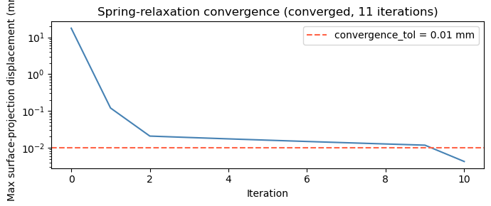
Converged: True  (11 iterations)

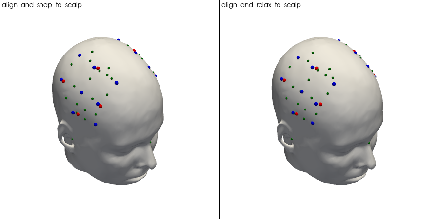
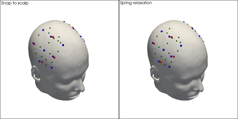
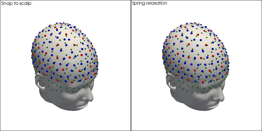
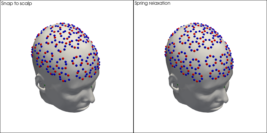
Visual comparison

Both registered montages are shown on the ICBM152 scalp surface. At this scale the two results look similar — the spring-relaxation differences are subtle in 3-D but become apparent in the channel-distance analysis below.

p = pv.Plotter(shape=(1, 2), window_size=(900, 450))

p.subplot(0, 0)
vbx.plot_surface(p, head_ras.scalp, color="w")
vbx.plot_labeled_points(p, geo3d_snapped)
p.add_text("align_and_snap_to_scalp", font_size=8)

p.subplot(0, 1)
vbx.plot_surface(p, head_ras.scalp, color="w")
vbx.plot_labeled_points(p, geo3d_relaxed)
p.add_text("align_and_relax_to_scalp", font_size=8)

p.show()

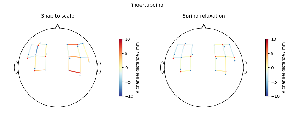
Channel distance changes

The color maps below show, for each channel, how much its source–detector distance changed after registration compared to the nominal (digitized) distances. Warm colors indicate elongated channels; cool colors indicate shortened channels.

Spring-relaxation should produce a map closer to zero overall — the springs resist large deviations from the nominal geometry.

nominal   = channel_distances(ts, geo3d)
d_snapped = (channel_distances(ts, geo3d_snapped) - nominal).pint.to("mm").pint.dequantify()
d_relaxed = (channel_distances(ts, geo3d_relaxed) - nominal).pint.to("mm").pint.dequantify()

fig, axes = plt.subplots(1, 2, figsize=(10, 4), dpi=100)

spargs = dict(
    vmin=-10, vmax=10,
    optode_size=2,
    cb_label="$\\Delta$ channel distance / mm",
    cmap=plt.cm.RdYlBu_r,
)
scalp_plot(ts, geo3d_snapped, d_snapped, axes[0], **spargs)
axes[0].set_title("Snap to scalp")

scalp_plot(ts, geo3d_relaxed, d_relaxed, axes[1], **spargs)
axes[1].set_title("Spring relaxation")

plt.tight_layout()
plt.show()

print(f"Snap   — mean |Δd|: {float(abs(d_snapped).mean()):.1f} mm, "
      f"max |Δd|: {float(abs(d_snapped).max()):.1f} mm")
print(f"Relax  — mean |Δd|: {float(abs(d_relaxed).mean()):.1f} mm, "
      f"max |Δd|: {float(abs(d_relaxed).max()):.1f} mm")

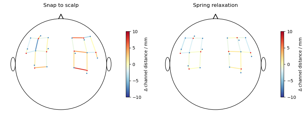
Snap   — mean |Δd|: 2.3 mm, max |Δd|: 7.6 mm
Relax  — mean |Δd|: 1.1 mm, max |Δd|: 2.9 mm

Convergence diagnostics

The SpringICPResult object returned by align_and_relax_to_scalp carries several quality-control metrics:

Attribute	Description
converged	True if the convergence criterion was met
n_iterations	Number of iterations actually performed
snap_displacement_per_iter	Max surface-projection displacement per iteration
spring_errors	Per-channel deviation from nominal distance at convergence
landmark_errors	Per-landmark distance to its anchor target at convergence

Convergence curve

The convergence curve shows the maximum projection displacement (the distance each optode had to travel to reach the scalp mesh after each force step). When this value drops below convergence_tol (default: 0.01 mm), the algorithm stops early.

fig, ax = plt.subplots(figsize=(7, 3), dpi=100)
ax.semilogy(details.snap_displacement_per_iter, color="steelblue")
ax.axhline(0.01, color="tomato", linestyle="--", label="convergence_tol = 0.01 mm")
ax.set_xlabel("Iteration")
ax.set_ylabel("Max surface-projection displacement (mm)")
ax.set_title(
    f"Spring-relaxation convergence "
    f"({'converged' if details.converged else 'did not converge'}, "
    f"{details.n_iterations} iterations)"
)
ax.legend()
plt.tight_layout()
plt.show()

Per-channel spring errors

Spring errors are the signed deviations of the final source–detector distances from the nominal (digitized) distances. Values close to zero mean the registration faithfully preserved the probe geometry. Large residuals indicate channels where the probe geometry conflicts with the scalp curvature.

spring_err = details.spring_errors  # xr.DataArray, dim: channel

fig, ax = plt.subplots(figsize=(10, 3), dpi=100)
ax.bar(range(len(spring_err)), spring_err.values,
       color=np.where(spring_err.values >= 0, "tomato", "steelblue"))
ax.axhline(0, color="k", linewidth=0.8)
ax.set_xlabel("Channel index")
ax.set_ylabel("Spring error (mm)")
ax.set_title("Per-channel deviation from nominal distance after registration")
plt.tight_layout()
plt.show()

print(f"Mean |spring error|: {float(abs(spring_err).mean()):.2f} mm")
print(f"Max  |spring error|: {float(abs(spring_err).max()):.2f} mm")

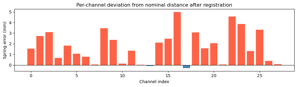
Mean |spring error|: 1.76 mm
Max  |spring error|: 5.00 mm

Landmark anchor errors

Landmark errors report how far each anchored landmark ended up from its target scalp position. These should be small (well below 1 mm with the default k_anchor = 10) — if they are large it may indicate a mismatch between the probe landmark labels and the atlas landmarks.

print("Landmark anchor errors at convergence:")
for lbl, err in zip(
    details.landmark_errors.label.values,
    details.landmark_errors.values,
):
    print(f"  {lbl:6s}: {err:.3f} mm")

Landmark anchor errors at convergence:
  LPA   : 2.586 mm
  Nz    : 0.758 mm
  RPA   : 3.927 mm

Algorithm parameters

The spring-relaxation algorithm has several tunable parameters:

Parameter	Default	Effect
n_iter	400	Maximum iterations before giving up
k_spring	1.0	Channel-spring stiffness — higher values push harder toward nominal distances
k_anchor	10.0	Landmark-anchor stiffness — keep above k_spring to enforce anatomical positions
step_size	0.1	Fraction of net force applied per step — lower values are more stable but slower
convergence_tol	0.01	Stop when max projection displacement < this value (mm)
initial_align_mode	"general"	Global alignment transform: "general" (affine, 12 DOF), "trans_rot_isoscale" (7 DOF), "trans_rot" (6 DOF), "identity"

For most use cases the defaults work well. If the algorithm reports that it did not converge within n_iter, try increasing n_iter or reducing step_size. If landmark errors are unexpectedly large, increase k_anchor.

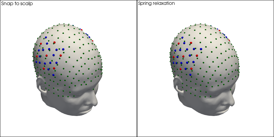
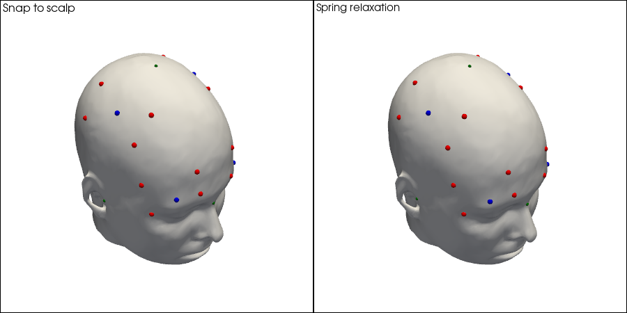
Comparison across multiple datasets

The cell below repeats the snap vs. relax comparison for all bundled test datasets. It provides a broader picture of how the two methods differ across probe designs ranging from sparse research arrays to ultra-high-density caps.

DATASETS = [
    "fingertapping",
    "fingertappingDOT",
    "nn22_resting",
    "ninja_cap_56x144",
    "ninja_uhd_cap_164x496",
    "lumo",
    "kernel",
    "artinis",
]


def get_fnirs_dataset(dataset):
    """Load geo3d, measurement list and time series for a named dataset."""
    if dataset == "fingertappingDOT":
        rec = cedalion.data.get_fingertappingDOT()
        return rec.geo3d, rec._measurement_lists["amp"], rec["amp"]
    elif dataset == "fingertapping":
        rec = cedalion.data.get_fingertapping()
        return rec.geo3d, rec._measurement_lists["amp"], rec["amp"]
    elif dataset == "nn22_resting":
        rec = cedalion.data.get_nn22_resting_state()
        return rec.geo3d, rec._measurement_lists["amp"], rec["amp"]
    elif dataset == "ninja_cap_56x144":
        geo3d, landmarks, meas_list = cedalion.data.get_ninja_cap_probe()
        geo3d = xr.concat((geo3d, landmarks), dim="label")
        geo3d = geo3d.pint.quantify("mm")
        ts = cedalion.dataclasses.empty_timeseries_from_measurement_list(meas_list)
        return geo3d, meas_list, ts
    elif dataset == "ninja_uhd_cap_164x496":
        geo3d, landmarks, meas_list = cedalion.data.get_ninja_uhd_cap_probe()
        geo3d = xr.concat((geo3d, landmarks), dim="label")
        geo3d = geo3d.pint.quantify("mm")
        ts = cedalion.dataclasses.empty_timeseries_from_measurement_list(meas_list)
        return geo3d, meas_list, ts
    elif dataset == "lumo":
        rec = cedalion.data.get_lumo_testdataset()
        geo3d = normalize_landmarks_labels(rec.geo3d)
        ch_mask = (
            channel_distances(rec["amp"], geo3d) < 3.5 * cedalion.units.cm
        )
        rec["amp"] = rec["amp"].sel(channel=ch_mask)
        return geo3d, rec._measurement_lists["amp"], rec["amp"]
    elif dataset == "artinis":
        rec = cedalion.data.get_artinis_testdataset()
        geo3d = normalize_landmarks_labels(rec.geo3d)
        geo3d = geo3d.pint.dequantify().pint.quantify("cm").pint.to("mm")
        # dataset lacks landmarks — borrow Colin27 landmarks
        head_ijk_c = cedalion.dot.get_standard_headmodel("colin27")
        head_ras_c = head_ijk_c.apply_transform(head_ijk_c.t_ijk2ras)
        colin_lm = head_ras_c.landmarks.sel(
            label=["Nz", "Iz", "LPA", "RPA", "Cz"]
        ).points.set_crs("pos")
        geo3d = xr.concat((geo3d, colin_lm), dim="label")
        return geo3d, rec._measurement_lists["amp"], rec["amp"]
    elif dataset == "kernel":
        rec = cedalion.data.get_kernel_testdataset()
        geo3d = normalize_landmarks_labels(rec.geo3d)
        return geo3d, rec._measurement_lists["amp"], rec["amp"]
    else:
        raise ValueError(f"Unknown dataset: {dataset}")


for dataset in DATASETS:
    print(f"\n{'='*60}\n{dataset}")
    head_ijk_d = cedalion.dot.get_standard_headmodel("icbm152")
    head_ras_d = head_ijk_d.apply_transform(head_ijk_d.t_ijk2ras)

    geo3d_d, meas_list_d, ts_d = get_fnirs_dataset(dataset)

    common_d = geo3d_d.points.common_labels(head_ras_d.landmarks)
    if len(common_d) > 3:
        mode_d = "general"
    elif len(common_d) == 3:
        mode_d = "trans_rot_isoscale"
    else:
        mode_d = "identity"

    geo3d_snapped_d = head_ras_d.align_and_snap_to_scalp(geo3d_d, mode=mode_d)
    geo3d_relaxed_d, details_d = head_ras_d.align_and_relax_to_scalp(
        geo3d_d, ts_d, initial_align_mode=mode_d
    )

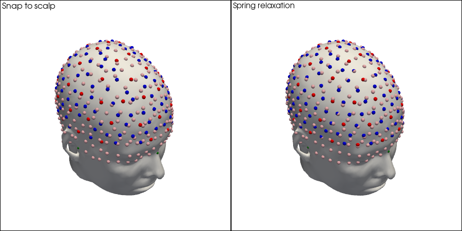
    # 3-D side-by-side
    p = pv.Plotter(shape=(1, 2), window_size=(900, 450))
    p.subplot(0, 0)
    vbx.plot_surface(p, head_ras_d.scalp, color="w")
    vbx.plot_labeled_points(p, geo3d_snapped_d)
    p.add_text("Snap to scalp", font_size=8)
    p.subplot(0, 1)
    vbx.plot_surface(p, head_ras_d.scalp, color="w")
    vbx.plot_labeled_points(p, geo3d_relaxed_d)
    p.add_text("Spring relaxation", font_size=8)
    p.show()

    # Channel-distance change maps
    nom_d   = channel_distances(ts_d, geo3d_d)
    d_sn_d  = (channel_distances(ts_d, geo3d_snapped_d) - nom_d).pint.to("mm").pint.dequantify()
    d_rl_d  = (channel_distances(ts_d, geo3d_relaxed_d) - nom_d).pint.to("mm").pint.dequantify()

    fig, axes = plt.subplots(1, 2, figsize=(10, 4), dpi=100)
    spargs = dict(
        vmin=-10, vmax=10, optode_size=2,
        cb_label="$\\Delta$ channel distance / mm",
        cmap=plt.cm.RdYlBu_r,
    )
    scalp_plot(ts_d, geo3d_snapped_d, d_sn_d, axes[0], **spargs)
    axes[0].set_title("Snap to scalp")
    scalp_plot(ts_d, geo3d_relaxed_d, d_rl_d, axes[1], **spargs)
    axes[1].set_title("Spring relaxation")
    fig.suptitle(dataset)
    plt.tight_layout()
    display(fig)
    plt.close(fig)

    print(f"  Snap:  mean |Δd| = {float(abs(d_sn_d).mean()):.1f} mm, "
          f"max = {float(abs(d_sn_d).max()):.1f} mm")
    print(f"  Relax: mean |Δd| = {float(abs(d_rl_d).mean()):.1f} mm, "
          f"max = {float(abs(d_rl_d).max()):.1f} mm  "
          f"({'converged' if details_d.converged else 'did not converge'}, "
          f"{details_d.n_iterations} iter)")

============================================================
fingertapping

  Snap:  mean |Δd| = 2.3 mm, max = 7.6 mm
  Relax: mean |Δd| = 1.1 mm, max = 2.9 mm  (converged, 11 iter)

============================================================
fingertappingDOT

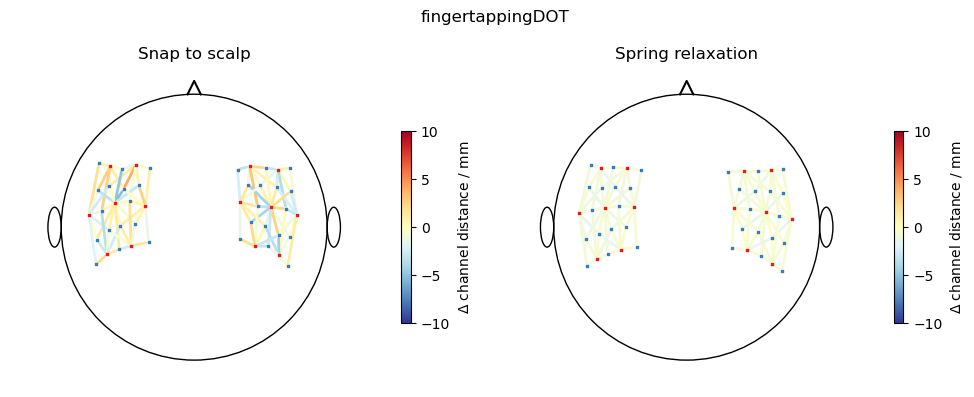
  Snap:  mean |Δd| = 1.7 mm, max = 5.2 mm
  Relax: mean |Δd| = 0.8 mm, max = 1.7 mm  (converged, 3 iter)

============================================================
nn22_resting

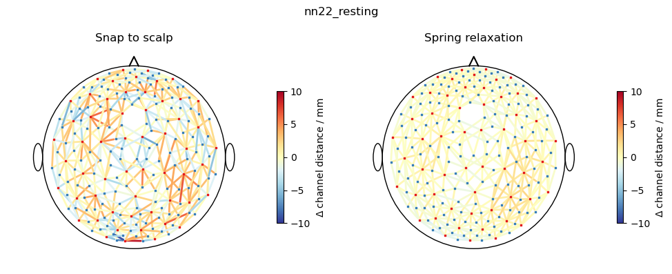
  Snap:  mean |Δd| = 1.9 mm, max = 9.1 mm
  Relax: mean |Δd| = 0.5 mm, max = 2.3 mm  (converged, 4 iter)

============================================================
ninja_cap_56x144

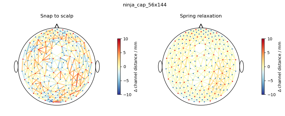
  Snap:  mean |Δd| = 1.9 mm, max = 9.1 mm
  Relax: mean |Δd| = 0.5 mm, max = 2.3 mm  (converged, 4 iter)

============================================================
ninja_uhd_cap_164x496

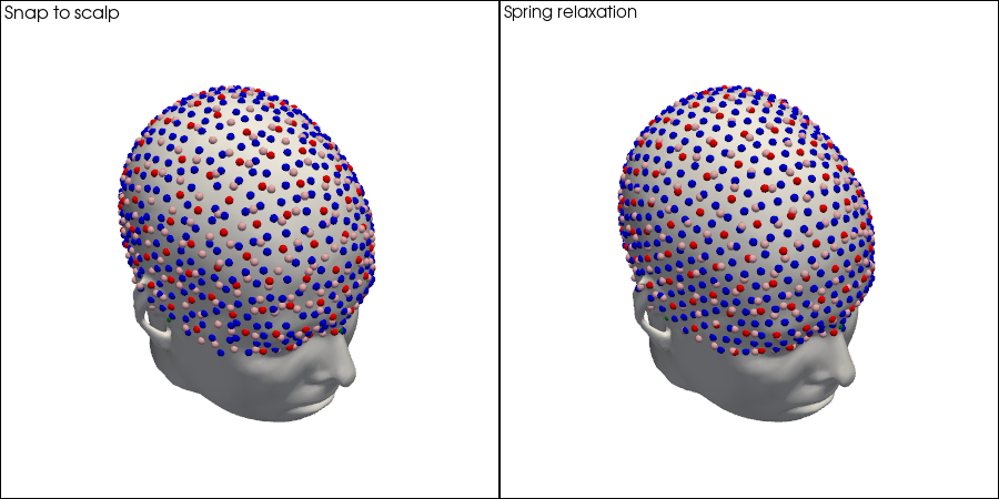
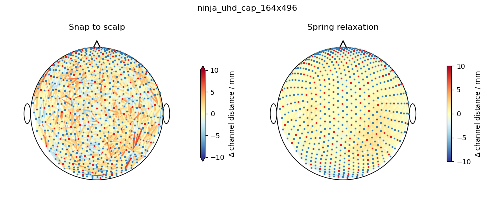
  Snap:  mean |Δd| = 1.7 mm, max = 12.3 mm
  Relax: mean |Δd| = 0.5 mm, max = 3.0 mm  (converged, 16 iter)

============================================================
lumo

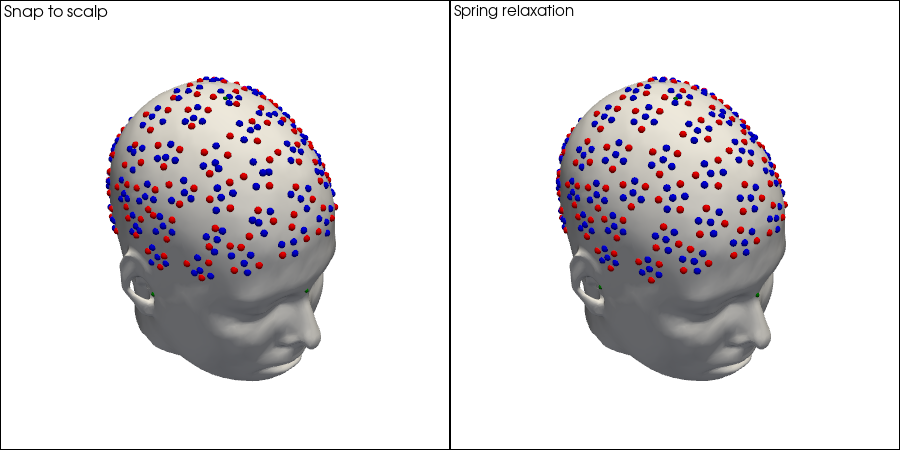
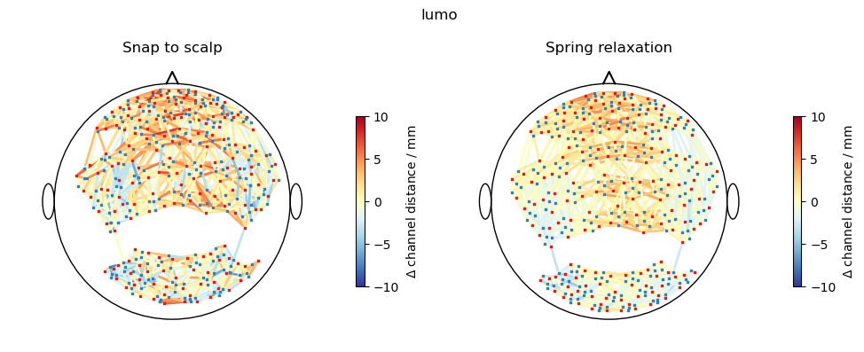
  Snap:  mean |Δd| = 2.0 mm, max = 8.3 mm
  Relax: mean |Δd| = 1.1 mm, max = 6.1 mm  (converged, 7 iter)

============================================================
kernel

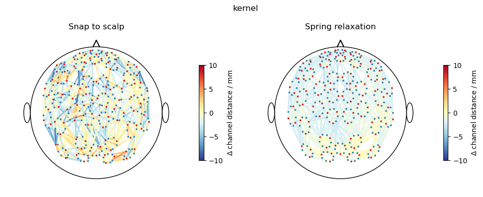
  Snap:  mean |Δd| = 1.9 mm, max = 7.7 mm
  Relax: mean |Δd| = 1.3 mm, max = 3.4 mm  (converged, 5 iter)

============================================================
artinis

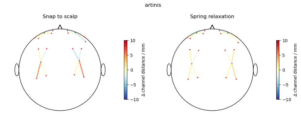
  Snap:  mean |Δd| = 1.7 mm, max = 5.6 mm
  Relax: mean |Δd| = 0.9 mm, max = 2.3 mm  (converged, 4 iter)

Summary

• Snap-to-scalp is fast and requires only landmark information, but can introduce noticeable channel-distance errors, especially for probes with tightly spaced optodes or probes placed over highly curved scalp regions.

• Spring-relaxation ICP preserves channel geometry by coupling source–detector pairs. It is slightly slower but typically yields smaller channel-distance deviations, especially for high-density arrays.

• The returned SpringICPResult object provides per-channel spring errors and a convergence curve that can be used as quality-control metrics.

Where to go next

• 43a_head_models_overview.ipynb — introduction to head models in Cedalion

• 41_photogrammetric_optode_coregistration.ipynb — registering photogrammetry-based optode positions

• 40_image_reconstruction.ipynb — using registered optodes for DOT image reconstruction