GLM Illustrative Example
This notebook explores cedalion’s GLM functionality. Using simulated timeseries with a known ‘ground truth’ allows us to clearly see how the GLM works. We fit several different models to the timeseries and showcase the GLM statistics afforded by cedalion’s statsmodels integration.
[1]:
# This cells setups the environment when executed in Google Colab.
try:
    import google.colab
    !curl -s https://raw.githubusercontent.com/ibs-lab/cedalion/dev/scripts/colab_setup.py -o colab_setup.py
    # Select branch with --branch "branch name" (default is "dev")
    %run colab_setup.py
except ImportError:
    pass
[2]:
import cedalion
import cedalion.io
import cedalion.nirs
import cedalion.dataclasses as cdc
import cedalion.models.glm as glm
import cedalion.vis.blocks as vbx
import cedalion.vis.anatomy
import numpy as np
import xarray as xr
import matplotlib.pyplot as p
import pandas as pd
from cedalion import units
from cedalion.sim.synthetic_hrf import RandomGaussianSum
xr.set_options(display_expand_data=False)
[2]:
<xarray.core.options.set_options at 0x7f6519c3d550>
Creating a simple simulated timeseries
In this section, we simulate an fNIRS timeseries by generating some random noise and then adding a simple HRF regressor.
1. Build a NDTimeSeries with noise
First, we’ll use the utility function build_timeseries to create a timeseries containing normally distributed noise. The build_timeseries function takes the following arguments:
data : The data values.
dims : The dimension names.
time : The time values.
channel : The channel names.
value_units : The units of the data values.
time_units : The units of the time values.
other_coords : dict[str, ArrayLike] Additional coordinates
[3]:
fs = 10.0 * cedalion.units.Hz # sampling rate
T = 240 * cedalion.units.s # time series length
channel = ["S1D1", "S1D2"] # two channels
chromo = ["HbO", "HbR"] # two chromophores
nsample = int(T * fs)  # number of samples

# create a NDTimeSeries that contains normal distributed noise
ts = cdc.build_timeseries(
    np.random.normal(0, 0.1, (nsample, len(channel), len(chromo))),
    dims=["time", "channel", "chromo"],
    time=np.arange(nsample) / fs,
    channel=channel,
    value_units=units.uM,
    time_units=units.s,
    other_coords={"chromo": chromo},
)
display(ts)
<xarray.DataArray (time: 2400, channel: 2, chromo: 2)> Size: 77kB
[µM] -0.001398 0.07036 -0.04387 -0.00274 ... 0.02757 0.1264 -0.03214 -0.1411
Coordinates:
  * time     (time) float64 19kB 0.0 0.1 0.2 0.3 0.4 ... 239.6 239.7 239.8 239.9
    samples  (time) int64 19kB 0 1 2 3 4 5 6 ... 2394 2395 2396 2397 2398 2399
  * channel  (channel) <U4 32B 'S1D1' 'S1D2'
* chromo (chromo) <U3 24B 'HbO' 'HbR'2. Build the Stimulus DataFrame
A stimulus Dataframe contains information about the experimental stimuli. It should have columns ‘trial_type’, ‘onset’, ‘duration’ and ‘value’.
In this example, we specify two trial types: ‘StimA’, ‘StimB’ and define for each 3 trials with a duration of 10s.
The trials get different values assigned, which we’ll use to control the amplitude of the hemodynamic response.
[4]:
stim = pd.concat(
    (
        pd.DataFrame({"onset": o, "trial_type": "StimA"} for o in [10, 80, 150]),
        pd.DataFrame({"onset": o, "trial_type": "StimB"} for o in [45, 115, 185]),
    )
)

stim["value"] = [0.5, 1, 1.5, 1.25, 0.75, 1.0]
stim["duration"] = 10.
display(stim)
| onset | trial_type | value | duration | |
|---|---|---|---|---|
| 0 | 10 | StimA | 0.50 | 10.0 |
| 1 | 80 | StimA | 1.00 | 10.0 |
| 2 | 150 | StimA | 1.50 | 10.0 |
| 0 | 45 | StimB | 1.25 | 10.0 |
| 1 | 115 | StimB | 0.75 | 10.0 |
| 2 | 185 | StimB | 1.00 | 10.0 |
3. Build a Design Matrix
We’ll use cedalion’s design matrix functionality to create a simulated HRF function that we can add to our timeseries.
We build a design matrix by concatenating different regressors. The regressor functions are found in glm.design_matrix. A regressor or sum of regressors returns a DesignMatrix object with two attributes:
common (xr.DataArray): regressors that apply to all channels, e.g. - HRF regressors - drift regressors - constant term
channel_wise (list[xr.DataArray]): regressors that can differ between channels. The motivating use-case is short-distance channel regression, in which one describes superficial components in long channels with a regressor made from a nearby short channel.
The functional form of the HRF regressors is specified by the basis_function argument. Please refer to the notebook glm_basis_functions.ipynb and the documentation for more details. In this section, we use the Gamma basis function, which takes these arguments:
tau: specifies a delay of the response with respect ot stimulus onset time.
sigma: specifies the width of the hemodynamic reponse.
T: If > 0, the response is additionally convoluted by a square wave of this width.
DesignMatrix.common stores regressors in an xr.DataArray with dimensions ‘time’, ‘chromo’ (or ‘wavelength’) and ‘regressor’.
Each regressor has a string label for clarity. The convention used by cedalion regressor functions is to use labels of the form 'HRF <trial_typ> <number>' for the HRF regressors and 'Drift <number>' for the drift components.
Using such a schema is convenient when one needs to select regressors. If there would be multiple regressors for stimulus “StimA” one could distinguish all these from other HRF or drift regressors by selecting labels that start with ‘HRF StimA’.
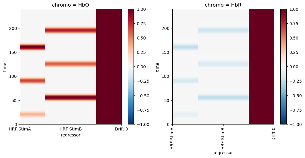
[5]:
# Design matrix built by concatenating the HRF and drift regressors
dms = (
glm.design_matrix.hrf_regressors(
ts, stim, glm.Gamma(tau=0 * units.s, sigma=5 * units.s)
)
& glm.design_matrix.drift_regressors(ts, drift_order=0)
)
display(dms.common)
dm = dms.common # there are no channel-wise regressors in this example
# For this use case we want the HbR regressors to be
# inverted and smaller in amplitude than their HbO counterparts.
dm.loc[:, ["HRF StimA", "HRF StimB"], "HbR"] *= -0.25
# Plot the design matrix/regressors
f, ax = p.subplots(1,2,figsize=(12,5))
dm.sel(chromo="HbO").plot(ax=ax[0], vmin=-1, vmax=1, cmap='RdBu_r')
dm.sel(chromo="HbR").plot(ax=ax[1], vmin=-1, vmax=1, cmap='RdBu_r')
p.xticks(rotation=90)
p.show()
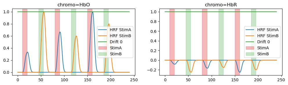
f, ax = p.subplots(1,2,figsize=(12,3))
for i,chromo in enumerate(dm.chromo.values):
for reg in dm.regressor.values:
ax[i].plot(dm.time, dm.sel(chromo=chromo, regressor=reg), label=reg)
vbx.plot_stim_markers(ax[i], stim, y=1)
ax[i].set_title(f"chromo={chromo}")
ax[i].legend()
<xarray.DataArray (time: 2400, regressor: 3, chromo: 2)> Size: 115kB
0.0 0.0 0.0 0.0 1.0 1.0 0.0 0.0 0.0 0.0 ... 0.0 1.0 1.0 0.0 0.0 0.0 0.0 1.0 1.0
Coordinates:
  * time       (time) float64 19kB 0.0 0.1 0.2 0.3 ... 239.6 239.7 239.8 239.9
  * regressor  (regressor) <U9 108B 'HRF StimA' 'HRF StimB' 'Drift 0'
  * chromo     (chromo) <U3 24B 'HbO' 'HbR'
4. Add regressors to time series with noise
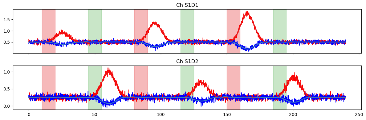
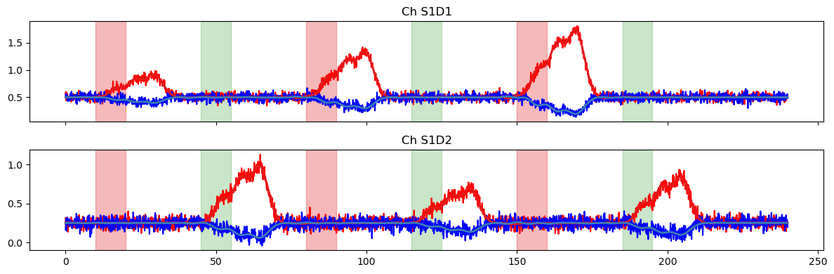
The time series has two channels: ‘S1D1’ and ‘S1D2’. In this toy example the stimuli will correspond to distinct channels: activations from trial ‘StimA’ should occur only in ‘S1D1’, and ‘StimB’ activations occur only in ‘S1D2’.
The regressors are added with different offsets and scaling factors, which determine the amplitude of the function. Later on we will compare our GLM results to these ‘ground truth’ amplitude values.
[6]:
# define offsets and scaling factors
SCALE_STIMA = 1.25
OFFSET_STIMA = 0.5
SCALE_STIMB = 0.75
OFFSET_STIMB = 0.25
# add scaled regressor and offsets to time series, which up to now contains only noise
ts.loc[:, "S1D1", :] += (
SCALE_STIMA * dm.sel(regressor="HRF StimA").pint.quantify("uM")
+ OFFSET_STIMA * cedalion.units.uM
)
ts.loc[:, "S1D2", :] += (
SCALE_STIMB * dm.sel(regressor="HRF StimB").pint.quantify("uM")
+ OFFSET_STIMB * cedalion.units.uM
)
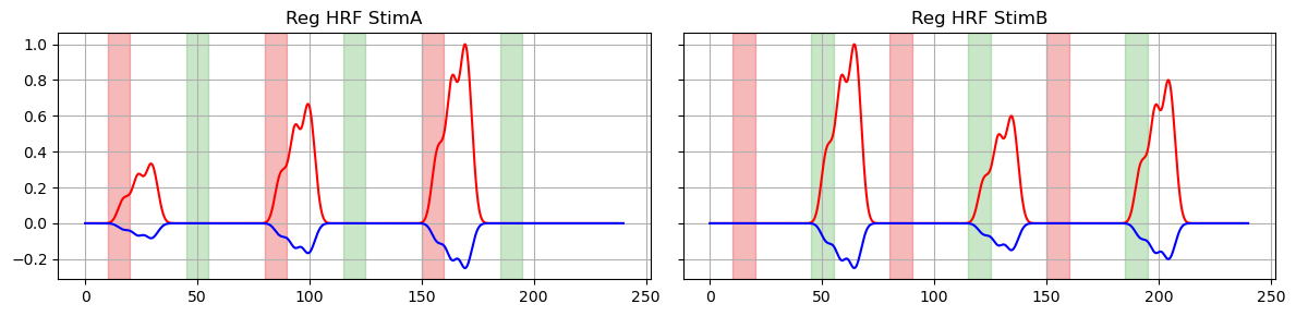
# plot original regressors for StimA and StimB
f, ax = p.subplots(1, 2, sharex=True, sharey=True, figsize=(12,3))
for i, reg in enumerate(["HRF StimA", "HRF StimB"]):
ax[i].plot(dm.time, dm.sel(regressor=reg, chromo="HbO"), "r-")
ax[i].plot(dm.time, dm.sel(regressor=reg, chromo="HbR"), "b-")
ax[i].set_title(f"Reg {reg}")
vbx.plot_stim_markers(ax[i], stim, y=1)
ax[i].grid(True)
p.tight_layout()
# plot the resulting time series
f, ax = p.subplots(1, 2, sharex=True, sharey=True, figsize=(12,3))
for i, ch in enumerate(ts.channel.values):
ax[i].plot(ts.time, ts.sel(channel=ch, chromo="HbO"), "r-")
ax[i].plot(ts.time, ts.sel(channel=ch, chromo="HbR"), "b-")
ax[i].set_title(f"Ch {ch}")
ax[i].grid(True)
vbx.plot_stim_markers(ax[i], stim, y=1)
p.tight_layout()

Fitting the GLM - using the same design matrix
In this section, we’ll fit our simulated timeseries using the same design matrix that we used to create it, just to make sure that everything is working as expected.
The method glm.fit is used to fit the GLM to the time series. The required arguments are timeseries and design matrix. We can optionally specify the noise model from the following currently available options:
ols (default): ordinary least squares
rls: recursive least squares
wls: weighted least squares
ar_irls: autoregressive iteratively reweighted least squares [BAH13]
gls: generalized least squares
glsar: generalized least squares with autoregressive covariance structure
The fit method returns an xr.DataArray of statsmodels RegressionResults objects with dimensions (channel, chromo). Any RegressionResults method can be called on this DataArray using the .sm accessor. For example, we access the betas or model coefficients by using result.sm.params. Please refer to the statsmodels documentation for a full list of methods and
attributes.
[7]:
result = glm.fit(ts, dms, noise_model="ols")
display(result)
 50%|█████     | 1/2 [00:00<00:00, 390.20it/s]
 50%|█████     | 1/2 [00:00<00:00, 79.63it/s]
<xarray.DataArray (channel: 2, chromo: 2)> Size: 32B
<statsmodels.regression.linear_model.RegressionResultsWrapper object at 0x7f6...
Coordinates:
  * channel  (channel) <U4 32B 'S1D1' 'S1D2'
  * chromo   (chromo) <U3 24B 'HbO' 'HbR'
Attributes:
description: OLS model via statsmodels.regression[8]:
betas = result.sm.params
betas
[8]:
<xarray.DataArray (channel: 2, chromo: 2, regressor: 3)> Size: 96B
1.25 -0.0001135 0.5045 1.251 0.0005666 ... 0.7499 0.2524 0.0004392 0.7497 0.2509
Coordinates:
  * regressor  (regressor) object 24B 'HRF StimA' 'HRF StimB' 'Drift 0'
  * channel    (channel) <U4 32B 'S1D1' 'S1D2'
  * chromo     (chromo) <U3 24B 'HbO' 'HbR'
Attributes:
description: OLS model via statsmodels.regressionNext, we’ll display our coefficiients in table.
The weights of the fitted model should correspond to the amplitudes of our original timeseries, which we know are just the scaling factors and offsets that we used above. We’ll add these amplitude values in an additional column.
[9]:
df = betas.rename("betas_S1D1").to_dataframe()
# add a column with expected values
df["Expected"] = [
    SCALE_STIMA, 0.0, OFFSET_STIMA,
    SCALE_STIMA, 0.0, OFFSET_STIMA,
    0.0, SCALE_STIMB, OFFSET_STIMB,
    0.0, SCALE_STIMB, OFFSET_STIMB,
]

display(df)
| betas_S1D1 | Expected | |||
|---|---|---|---|---|
| channel | chromo | regressor | ||
| S1D1 | HbO | HRF StimA | 1.249968 | 1.25 |
| HRF StimB | -0.000114 | 0.00 | ||
| Drift 0 | 0.504481 | 0.50 | ||
| HbR | HRF StimA | 1.251191 | 1.25 | |
| HRF StimB | 0.000567 | 0.00 | ||
| Drift 0 | 0.500949 | 0.50 | ||
| S1D2 | HbO | HRF StimA | 0.000063 | 0.00 |
| HRF StimB | 0.749909 | 0.75 | ||
| Drift 0 | 0.252391 | 0.25 | ||
| HbR | HRF StimA | 0.000439 | 0.00 | |
| HRF StimB | 0.749732 | 0.75 | ||
| Drift 0 | 0.250856 | 0.25 |
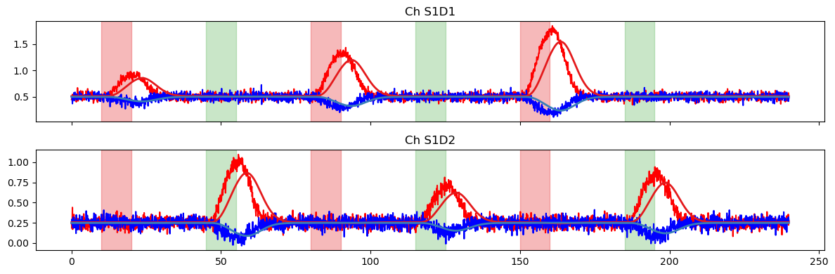
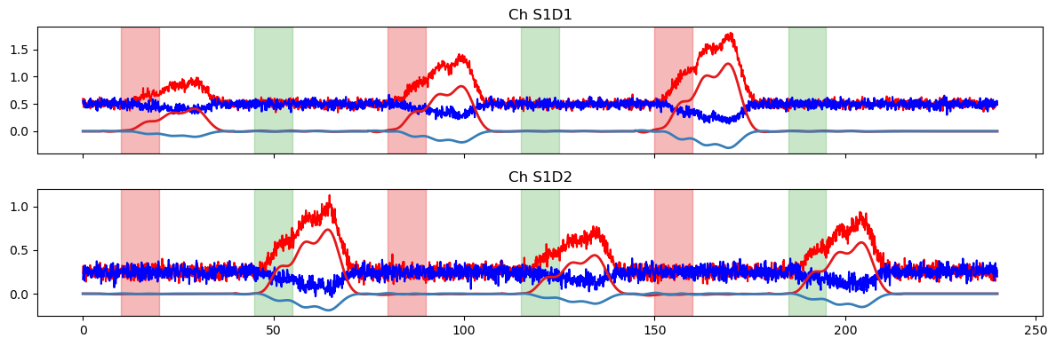
Finally, we use the design matrix and fitted coefficients to predict the timeseries using glm.predict.
[10]:
# helper function to compare original time series and model prediction
def plot_data_to_fit_comparison(ts, pred, stim):
f, ax = p.subplots(2,1, sharex=True, figsize=(12,4))
for i, ch in enumerate(ts.channel.values):
ax[i].plot(ts.time, ts.sel(channel=ch, chromo="HbO"), "r-")
ax[i].plot(ts.time, ts.sel(channel=ch, chromo="HbR"), "b-")
ax[i].plot(pred.time, pred.sel(channel=ch, chromo="HbO"), "-", c="#e41a1c", lw=2)
ax[i].plot(pred.time, pred.sel(channel=ch, chromo="HbR"), "-", c="#377eb8", lw=2)
ax[i].set_title(f"Ch {ch}")
vbx.plot_stim_markers(ax[i], stim, y=1)
p.tight_layout()
# use all regressors of the design matrix to predict the time series
pred = glm.predict(ts, betas, dms)
display(pred)
plot_data_to_fit_comparison(ts, pred, stim)
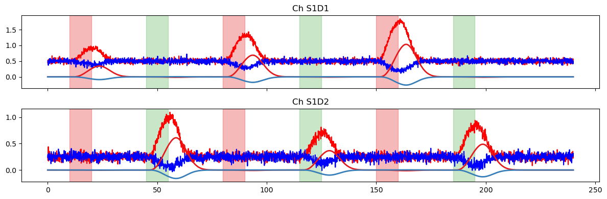
# use only HRF-related regressors, i.e. remove the drift/offset
pred = glm.predict(
ts,
# select regressor whose label start with HRF Stim
betas.sel(regressor=betas.regressor.str.startswith("HRF Stim")),
dms
)
plot_data_to_fit_comparison(ts, pred, stim)
<xarray.DataArray (time: 2400, channel: 2, chromo: 2)> Size: 77kB
0.5045 0.5009 0.2524 0.2509 0.5045 0.5009 ... 0.2509 0.5045 0.5009 0.2524 0.2509
Coordinates:
  * time     (time) float64 19kB 0.0 0.1 0.2 0.3 0.4 ... 239.6 239.7 239.8 239.9
  * chromo   (chromo) <U3 24B 'HbO' 'HbR'
  * channel  (channel) <U4 32B 'S1D1' 'S1D2'

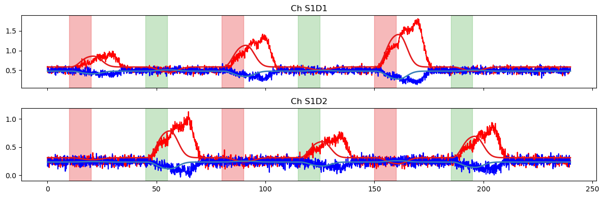
Fitting the GLM - this time using a slightly different model
In this section, we create a new design matrix that encodes less prior knowledge about the timeseries.
[11]:
# copy the stimulus DataFrame and set all values to 1, i.e.
# there is no prior knowledge about amplitude differences between trials
stim_other = stim.copy()
stim_other["value"] = 1.
display(stim_other)

# this design matrix also uses Gamma basis functions but
# the onset (tau) is delayed and the HRF width (sigma) is longer.
dms_other = (
    glm.design_matrix.hrf_regressors(
        ts, stim, glm.Gamma(tau=1 * units.s, sigma=7 * units.s)
    )
    & glm.design_matrix.drift_regressors(ts, drift_order=0)
)


betas = glm.fit(ts, dms_other, noise_model="ols").sm.params

# display the fitted betas as a DataFrame
display(betas.rename("betas_S1D1").to_dataframe())
| onset | trial_type | value | duration | |
|---|---|---|---|---|
| 0 | 10 | StimA | 1.0 | 10.0 |
| 1 | 80 | StimA | 1.0 | 10.0 |
| 2 | 150 | StimA | 1.0 | 10.0 |
| 0 | 45 | StimB | 1.0 | 10.0 |
| 1 | 115 | StimB | 1.0 | 10.0 |
| 2 | 185 | StimB | 1.0 | 10.0 |
 50%|█████     | 1/2 [00:00<00:00, 301.29it/s]
 50%|█████     | 1/2 [00:00<00:00, 83.66it/s]
| betas_S1D1 | |||
|---|---|---|---|
| channel | chromo | regressor | |
| S1D1 | HbO | HRF StimA | 0.822069 |
| HRF StimB | -0.016721 | ||
| Drift 0 | 1.425679 | ||
| HbR | HRF StimA | -0.205697 | |
| HRF StimB | 0.004019 | ||
| Drift 0 | 0.270652 | ||
| S1D2 | HbO | HRF StimA | -0.008895 |
| HRF StimB | 0.492026 | ||
| Drift 0 | 0.806378 | ||
| HbR | HRF StimA | 0.002204 | |
| HRF StimB | -0.122945 | ||
| Drift 0 | 0.111546 |
[12]:
pred = glm.predict(ts, betas, dms_other)
display(pred)
plot_data_to_fit_comparison(ts, pred, stim_other)


pred = glm.predict(
    ts,
    betas.sel(regressor=betas.regressor.str.startswith("HRF Stim")),
    dms_other
)
plot_data_to_fit_comparison(ts, pred, stim_other)
<xarray.DataArray (time: 2400, channel: 2, chromo: 2)> Size: 77kB
1.426 0.2707 0.8064 0.1115 1.426 0.2707 ... 0.1115 1.426 0.2707 0.8064 0.1115
Coordinates:
  * time     (time) float64 19kB 0.0 0.1 0.2 0.3 0.4 ... 239.6 239.7 239.8 239.9
  * chromo   (chromo) <U3 24B 'HbO' 'HbR'
  * channel  (channel) <U4 32B 'S1D1' 'S1D2'
Creating a new, more complicated time series
In this section, we’ll build a more complicated simulated HRF, following the same steps as in the first part of this notebook. The only thing we do differently is pass a different basis function (RandomGaussianSum) to glm.design_matrix.hrf_regressors.
[13]:
fs = 10.0 * cedalion.units.Hz # sampling rate
T = 240 * cedalion.units.s # time series length
channel = ["S1D1", "S1D2"] # two channels
chromo = ["HbO", "HbR"] # two chromophores
nsample = int(T * fs) # number of samples
# create a NDTimeSeries that contains normal distributed noise
ts = cdc.build_timeseries(
np.random.normal(0, 0.1, (nsample, len(channel), len(chromo))),
dims=["time", "channel", "chromo"],
time=np.arange(nsample) / fs,
channel=channel,
value_units=units.uM,
time_units=units.s,
other_coords={"chromo": chromo},
)
# Create a design matrix with a random Gaussian sum HRF
dms = (
glm.design_matrix.hrf_regressors(
ts, stim, RandomGaussianSum(
t_start=0 * units.s,
t_end=30 * units.s,
t_delta=2 * units.s,
t_std=3 * units.s,
seed=22,
)
)
& glm.design_matrix.drift_regressors(ts, drift_order=0)
)
dm = dms.common # there are no channel-wise regressors in this example
# For this simulated example we again want the HbR regressors to be
# inverted and smaller in amplitude than their HbO counterparts.
dm.loc[:, ["HRF StimA", "HRF StimB"], "HbR"] *= -0.25
# define offsets and scaling factors
SCALE_STIMA = 1.25
OFFSET_STIMA = 0.5
SCALE_STIMB = 0.75
OFFSET_STIMB = 0.25
# add scaled regressor and offsets to time series, which up to now contains only noise
ts.loc[:, "S1D1", :] += (
SCALE_STIMA * dm.sel(regressor="HRF StimA").pint.quantify("uM")
+ OFFSET_STIMA * cedalion.units.uM
)
ts.loc[:, "S1D2", :] += (
SCALE_STIMB * dm.sel(regressor="HRF StimB").pint.quantify("uM")
+ OFFSET_STIMB * cedalion.units.uM
)
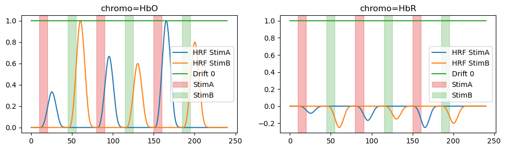
# plot original regressors for StimA and StimB
f, ax = p.subplots(1, 2, sharex=True, sharey=True, figsize=(12,3))
for i, reg in enumerate(["HRF StimA", "HRF StimB"]):
ax[i].plot(dm.time, dm.sel(regressor=reg, chromo="HbO"), "r-")
ax[i].plot(dm.time, dm.sel(regressor=reg, chromo="HbR"), "b-")
ax[i].set_title(f"Reg {reg}")
vbx.plot_stim_markers(ax[i], stim, y=1)
ax[i].grid(True)
p.tight_layout()
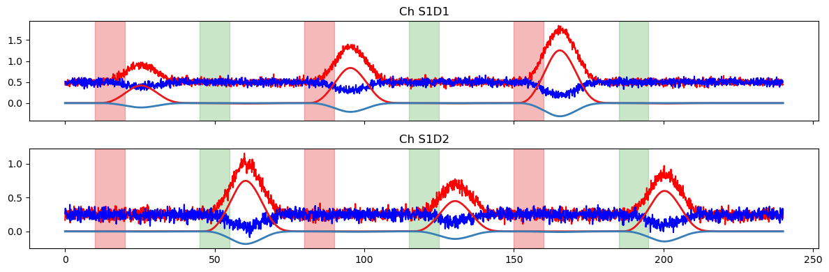
# plot the resulting time series
f, ax = p.subplots(1, 2, sharex=True, sharey=True, figsize=(12,3))
for i, ch in enumerate(ts.channel.values):
ax[i].plot(ts.time, ts.sel(channel=ch, chromo="HbO"), "r-")
ax[i].plot(ts.time, ts.sel(channel=ch, chromo="HbR"), "b-")
ax[i].set_title(f"Ch {ch}")
ax[i].grid(True)
vbx.plot_stim_markers(ax[i], stim, y=1)
p.tight_layout()
Fitting the GLM - Uncertainty
The aim of this section is to showcase some uncertainty measurements of the GLM fit that are accessible through statsmodels. First, we’ll create a simple design matrix using gamma basis functions, following the same steps as in the previous sections.
[14]:
dms_simple = (
    glm.design_matrix.hrf_regressors(
        ts, stim, glm.Gamma(tau=0 * units.s, sigma=5 * units.s)
    )
    & glm.design_matrix.drift_regressors(ts, drift_order=0)
)

dm_simple = dms_simple.common

dm_simple.loc[:, ["HRF StimA", "HRF StimB"], "HbR"] *= -0.25 # invert HbR regressors

f, ax = p.subplots(1,2,figsize=(12,5))
dm_simple.sel(chromo="HbO").plot(ax=ax[0], vmin=-1, vmax=1, cmap='RdBu_r')
dm_simple.sel(chromo="HbR").plot(ax=ax[1], vmin=-1, vmax=1, cmap='RdBu_r')
p.xticks(rotation=90)
p.show()

f, ax = p.subplots(1,2,figsize=(12,3))
for i,chromo in enumerate(dm_simple.chromo.values):
    for reg in dm_simple.regressor.values:
        ax[i].plot(dm_simple.time, dm_simple.sel(chromo=chromo, regressor=reg), label=reg)
    vbx.plot_stim_markers(ax[i], stim, y=1)
    ax[i].set_title(f"chromo={chromo}")
    ax[i].legend()

Now, we fit the GLM and showcase some useful uncertainty measures. As noted above, the glm.fit function returns a DataArray of statsmodels RegressionResults objects, and the full list of available methods can be found in the statsmodels documentation. Here, we calculate the standard error, variance, and confidence intervals of our GLM coefficients.
Even though our HRF is more complicated now, the weights of the fitted simple model should still roughly correspond to the max amplitudes of our original timeseries (TS Amplitude), which we know are just the scaling factors and offsets that we used above.
[15]:
# fit the model to the time series
result = glm.fit(ts, dms_simple, noise_model="ols")
betas = result.sm.params

# display the fitted betas as a DataFrame
df = betas.rename("betas_S1D1").to_dataframe()
# add a column with expected values
df["TS Amplitude"] = [
    SCALE_STIMA, 0.0, OFFSET_STIMA,
    SCALE_STIMA, 0.0, OFFSET_STIMA,
    0.0, SCALE_STIMB, OFFSET_STIMB,
    0.0, SCALE_STIMB, OFFSET_STIMB,
]

# calculate uncertainty measures and add to table
df["Standard Error"] = result.sm.bse.rename("Standard Error").to_dataframe() # standard error
conf_int_df = result.sm.conf_int().to_dataframe(name="conf_int").unstack() # confidence intervals
conf_int_df.columns = ["Confidence Interval Lower", "Confidence Interval Upper"]
df = df.join(conf_int_df)
df["Variance"] = result.sm.regressor_variances().rename("Variance").to_dataframe() # variance

# reorder columns
df = df[["TS Amplitude", "Confidence Interval Lower", "betas_S1D1", "Confidence Interval Upper", "Standard Error", "Variance"]]

display(df)
 50%|█████     | 1/2 [00:00<00:00, 79.37it/s]
 50%|█████     | 1/2 [00:00<00:00, 82.39it/s]
| TS Amplitude | Confidence Interval Lower | betas_S1D1 | Confidence Interval Upper | Standard Error | Variance | |||
|---|---|---|---|---|---|---|---|---|
| channel | chromo | regressor | ||||||
| S1D1 | HbO | HRF StimA | 1.25 | 0.013120 | 0.013862 | 0.014604 | 0.000378 | 1.432016e-07 |
| HRF StimB | 0.00 | -0.003745 | -0.002951 | -0.002158 | 0.000405 | 1.637529e-07 | ||
| Drift 0 | 0.50 | 0.610569 | 0.626542 | 0.642515 | 0.008146 | 6.635001e-05 | ||
| HbR | HRF StimA | 1.25 | 0.011940 | 0.013074 | 0.014207 | 0.000578 | 3.340802e-07 | |
| HRF StimB | 0.00 | -0.003456 | -0.002244 | -0.001032 | 0.000618 | 3.820250e-07 | ||
| Drift 0 | 0.50 | 0.457861 | 0.463960 | 0.470060 | 0.003110 | 9.674397e-06 | ||
| S1D2 | HbO | HRF StimA | 0.00 | -0.002092 | -0.001640 | -0.001187 | 0.000231 | 5.324384e-08 |
| HRF StimB | 0.75 | 0.007623 | 0.008107 | 0.008590 | 0.000247 | 6.088501e-08 | ||
| Drift 0 | 0.25 | 0.317039 | 0.326779 | 0.336518 | 0.004967 | 2.466962e-05 | ||
| HbR | HRF StimA | 0.00 | -0.002312 | -0.001301 | -0.000290 | 0.000516 | 2.658673e-07 | |
| HRF StimB | 0.75 | 0.006480 | 0.007561 | 0.008642 | 0.000551 | 3.040227e-07 | ||
| Drift 0 | 0.25 | 0.227274 | 0.232715 | 0.238156 | 0.002775 | 7.699068e-06 |
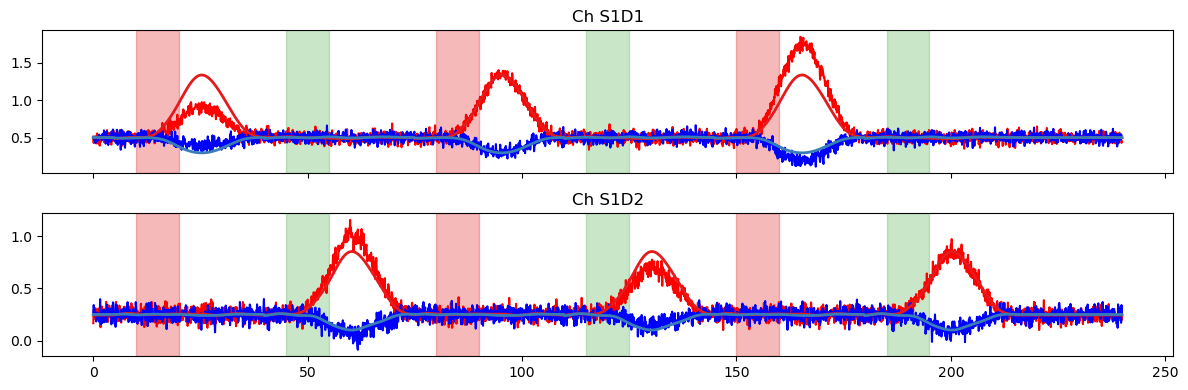
Next, we plot the model prediction and compare it to the time series.
[16]:
# use all regressors of the design matrix to predict the time series
pred = glm.predict(ts, betas, dms_simple)
display(pred)
plot_data_to_fit_comparison(ts, pred, stim)


# use only HRF-related regressors, i.e. remove the drift/offset
pred = glm.predict(
    ts,
    # select regressor whose label start with HRF Stim
    betas.sel(regressor=betas.regressor.str.startswith("HRF Stim")),
    dms_simple
)
plot_data_to_fit_comparison(ts, pred, stim)
<xarray.DataArray (time: 2400, channel: 2, chromo: 2)> Size: 77kB
0.6265 0.464 0.3268 0.2327 0.6265 0.464 ... 0.2327 0.6265 0.464 0.3268 0.2327
Coordinates:
  * time     (time) float64 19kB 0.0 0.1 0.2 0.3 0.4 ... 239.6 239.7 239.8 239.9
  * chromo   (chromo) <U3 24B 'HbO' 'HbR'
  * channel  (channel) <U4 32B 'S1D1' 'S1D2'
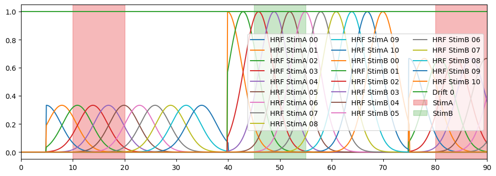
Fitting with multiple gaussian kernels
In this section, we’ll build a new design matrix using the GaussianKernels basis function. This basis function consists of multiple time-shifted gaussians. Therefore, the model is capable of describing also more complex hemodynamic repsonse - like the one we just simulated. However, the obtained coefficients are not as easy to interprete as in the simpler model above. There the size of the coefficient directly related to the amplitude of the response. Here, the coefficients of the Gaussians
encode both the shape and the amplitude.
The GaussianKernels basis function takes the following arguments:
t_pre : time before trial onset
t_post : time after trial onset
t_delta : the temporal spacing between consecutive gaussians
t_std : time width of the gaussians
[17]:
# Build design matrix with Gaussian kernels
gaussian_kernels = glm.GaussianKernels(
    t_pre=5 * units.s, t_post=30 * units.s, t_delta=3 * units.s, t_std=2 * units.s
)

dms_gauss = glm.design_matrix.hrf_regressors(
    ts,
    stim,
    gaussian_kernels,
) & glm.design_matrix.drift_regressors(ts, drift_order=0)

dm_gauss = dms_gauss.common

# Plot the regressors
f,ax = p.subplots(1,1, figsize=(12,4))
for reg in dm_gauss.regressor.values:
    p.plot(dm_gauss.time, dm_gauss.sel(chromo="HbO", regressor=reg), label=reg)
vbx.plot_stim_markers(ax, stim, y=1.)
p.legend(ncol=3, loc="center right")
p.xlim(0,90)
[17]:
(0.0, 90.0)
Now we use the new design matrix to fit the GLM.
Note that we have many regressors and thus no longer can easily infer the HRF amplitude from the coefficients. We also need a more sophisticated way to display the uncertainty of our fit.
[18]:
# Fit the model to the time series
results = glm.fit(ts, dms_gauss, noise_model="ols")
betas = results.sm.params

# translate the xr.DataArray into a pd.DataFrame which are displayed as tables
display(betas.rename("betas_S1D1").to_dataframe())
 50%|█████     | 1/2 [00:00<00:00,  4.01it/s]
 50%|█████     | 1/2 [00:00<00:00,  3.47it/s]
| betas_S1D1 | |||
|---|---|---|---|
| channel | chromo | regressor | |
| S1D1 | HbO | HRF StimA 00 | 0.117227 |
| HRF StimA 01 | -0.191155 | ||
| HRF StimA 02 | 0.285820 | ||
| HRF StimA 03 | -0.462502 | ||
| HRF StimA 04 | 1.037423 | ||
| ... | ... | ... | ... |
| S1D2 | HbR | HRF StimB 07 | 0.124788 |
| HRF StimB 08 | -0.238181 | ||
| HRF StimB 09 | 0.008895 | ||
| HRF StimB 10 | -0.011663 | ||
| Drift 0 | 0.255639 |
92 rows × 1 columns
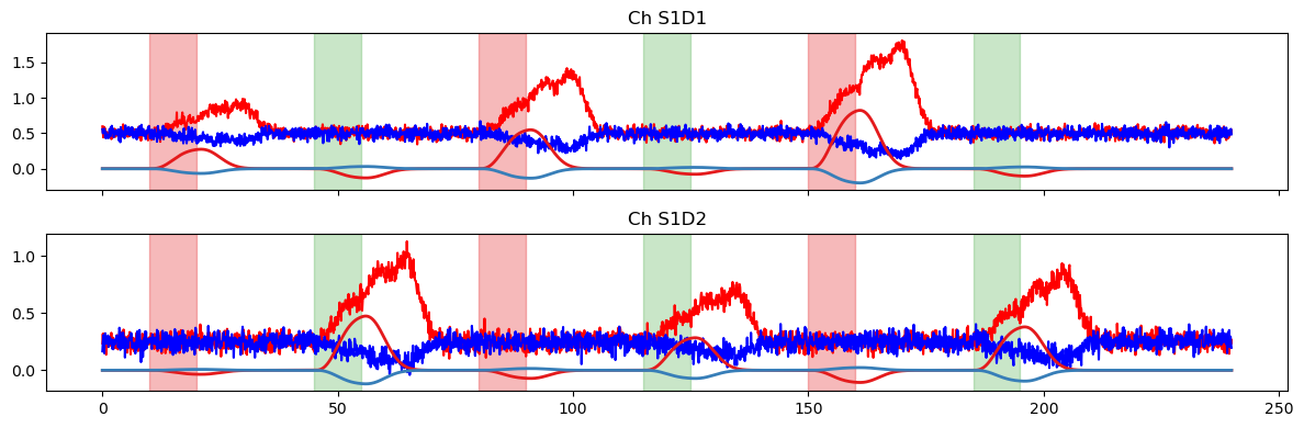
We again use the fitted model to predict the time series. This time, the prediction is quite accurate.
[19]:
pred = glm.predict(ts, betas, dms_gauss)
plot_data_to_fit_comparison(ts, pred, stim)


# use only HRF-related regressors, i.e. remove the drift/offset
pred_stim = glm.predict(
    ts,
    # select regressor whose label start with HRF Stim
    betas.sel(regressor=betas.regressor.str.startswith("HRF Stim")),
    dms_gauss
)
plot_data_to_fit_comparison(ts, pred_stim, stim)
In the last part of the notebook, we’ll explore some options for using a derived statistic to enable quantitative comparisons between the prediction and the original timeseries.
First, we compare the peak amplitude and area under the curve of the prediction and the original timeseries.
TODO: uncertainty measurements for these values
[20]:
# calculate peak amplitude and area under the curve (AUC) for each channel and chromophore
peak_amp_pred = pred.max(dim=["time"]).to_dataframe(name="peak_amp_pred")
auc_pred = pred.integrate(coord="time").to_dataframe(name="auc_pred")

# calculate peak amplitude and AUC for the original time series
peak_amp_ts = ts.pint.dequantify().max(dim=["time"]).to_dataframe(name="peak_amp_ts")
auc_ts = ts.pint.dequantify().integrate(coord="time").to_dataframe(name="auc_ts")

# merge the results into a single DataFrame and display
df = peak_amp_ts.join(peak_amp_pred).join(auc_ts).join(auc_pred)

display(df)
| peak_amp_ts | peak_amp_pred | auc_ts | auc_pred | ||
|---|---|---|---|---|---|
| channel | chromo | ||||
| S1D1 | HbO | 2.585659 | 2.367128 | 170.033481 | 170.032814 |
| HbR | 0.889501 | 0.522104 | 106.406437 | 106.409004 | |
| S1D2 | HbO | 1.465415 | 1.171906 | 90.083937 | 90.086131 |
| HbR | 0.624475 | 0.277867 | 53.007407 | 52.998469 |
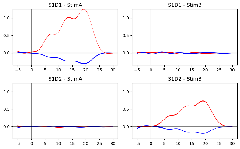
Finally, we try out a way to visualize the uncertainty of the GLM fit. In the simple case, we could just look at the uncertainties of each coefficient. Now that we have so many coefficients, this is no longer feasible.
This method visualizes the uncertainty in a GLM fit by drawing multiple samples of the beta coefficients from their estimated covariance (via multivariate normal sampling). It then uses these sampled betas to generate predicted time courses, and plots the mean prediction with a shaded band representing ±3 standard deviations across samples, thus capturing the variability due to model uncertainty. The band is quite narrow because uncertainty is low in this toy example.
[21]:
dms_extract = glm.design_matrix.hrf_extract_regressors(ts, stim, gaussian_kernels)
display(dms_extract.common)
<xarray.DataArray (time: 352, regressor: 22, chromo: 2)> Size: 124kB
1.0 1.0 0.5698 0.5698 0.1054 0.1054 ... 0.0004525 0.01656 0.01656 0.1968 0.1968
Coordinates:
  * time       (time) float64 3kB -5.1 -5.0 -4.9 -4.8 ... 29.7 29.8 29.9 30.0
  * regressor  (regressor) <U12 1kB 'HRF StimA 00' ... 'HRF StimB 10'
  * chromo     (chromo) <U3 24B 'HbO' 'HbR'
[22]:
results.sm.params.regressor.str.startswith("HRF Stim")
[22]:
<xarray.DataArray 'regressor' (regressor: 23)> Size: 23B
True True True True True True True True ... True True True True True True False
Coordinates:
  * regressor  (regressor) object 184B 'HRF StimA 00' ... 'Drift 0'
[23]:
ch = "S1D1"

f,ax = p.subplots(2,2, figsize=(8,5))


for i_c, trial in enumerate(["StimA", "StimB"]):
    # get mean prediction and the uncertainty band
    hrfs_mean, hrfs_std = glm.predict_with_uncertainty(
            ts,
            results,
            dms_extract,
            results.sm.params.regressor.str.startswith(f"HRF {trial}"),
        )

    # plot means and uncertainty bands for all trial types and channels
    for i_r, ch in enumerate(["S1D1", "S1D2"]):
        mm_hbo = hrfs_mean.sel(channel=ch, chromo="HbO")
        mm_hbr = hrfs_mean.sel(channel=ch, chromo="HbR")
        ss_hbo = hrfs_std.sel(channel=ch, chromo="HbO")
        ss_hbr = hrfs_std.sel(channel=ch, chromo="HbR")


        ax[i_r, i_c].fill_between(
            mm_hbo.time, mm_hbo - ss_hbo, mm_hbo + ss_hbo, fc="r", alpha=1
        )

        ax[i_r, i_c].fill_between(
            mm_hbr.time, mm_hbr - ss_hbr, mm_hbr + ss_hbr, fc="b", alpha=1
        )

        ax[i_r, i_c].set_ylim(-.35, 1.25)
        ax[i_r, i_c].set_title(f"{ch} - {trial}")
        ax[i_r, i_c].axhline(0, c="k", alpha=.5, zorder=1)
        ax[i_r, i_c].axvline(0, c="k", alpha=.5, zorder=1)
p.tight_layout()
References
[24]:
cedalion.bib.dump_to_notebook()
Methods used
| [1] | Strangman2002 | cedalion.models.glm.basis_functions.Gamma.__call__ | Gary Strangman, Joseph P. Culver, John H. Thompson, and David A. Boas. A quantitative comparison of simultaneous BOLD fMRI and NIRS recordings during functional brain activation. NeuroImage, 17(2):719–731, 2002. doi:10.1006/nimg.2002.1227. |
| [2] | Barker2013 | cedalion.models.glm.solve.fit | Jeffrey W. Barker, Ardalan Aarabi, and Theodore J. Huppert. Autoregressive model based algorithm for correcting motion and serially correlated errors in fnirs. Biomed. Opt. Express, 4(8):1366–1379, Aug 2013. doi:10.1364/BOE.4.001366. |