Xarray Data Structures - an fNIRS example

This exampple illustrates the usage of xarray-based data structures for calculating the Beer-Lambert transformation.

import cedalion
import cedalion.nirs
import cedalion.xrutils
import cedalion.xrutils as xrutils
from cedalion.datasets import get_fingertapping_snirf_path
import numpy as np
import xarray as xr
import pint
import matplotlib.pyplot as p
import scipy.signal
import os.path
xr.set_options(display_max_rows=3, display_values_threshold=50)
np.set_printoptions(precision=4)

Loading raw CW-NIRS data from a SNIRF file

This notebook uses a finger-tapping dataset in BIDS layout provided by Rob Luke. It can can be downloaded via cedalion.datasets.

Load amplitude data from the snirf file.

path_to_snirf_file = get_fingertapping_snirf_path()

recordings = cedalion.io.read_snirf(path_to_snirf_file)
rec = recordings[0] # there is only one NirsElement in this snirf file...
amp = rec["amp"]    # ... which holds amplitude data

# restrict to first 60 seconds and fill in missing units
amp = amp.sel(time=amp.time < 60)
amp = amp.pint.dequantify().pint.quantify("V")
geo3d = rec.geo3d

recordings

[<Recording |  timeseries: ['amp'],  masks: [],  stim: ['1.0', '15.0', '2.0', '3.0'],  aux_ts: [],  aux_obj: []>]

Amplitude data

display(amp.round(4))

<xarray.DataArray (channel: 28, wavelength: 2, time: 469)> Size: 210kB
<Quantity([[[0.0914 0.091  0.091  ... 0.0903 0.0902 0.0899]
  [0.1857 0.1864 0.1837 ... 0.1849 0.185  0.1847]]

 [[0.2275 0.2297 0.2261 ... 0.2241 0.2243 0.2257]
  [0.6355 0.6377 0.6298 ... 0.6223 0.6237 0.6272]]

 [[0.1065 0.1066 0.1053 ... 0.1065 0.1062 0.1056]
  [0.2755 0.2762 0.2727 ... 0.2737 0.2742 0.276 ]]

 ...

 [[0.2028 0.1997 0.2005 ... 0.1998 0.2007 0.2026]
  [0.4666 0.4554 0.4562 ... 0.4482 0.4511 0.4541]]

 [[0.4885 0.4802 0.4818 ... 0.5005 0.5036 0.5045]
  [0.8458 0.826  0.826  ... 0.8386 0.8441 0.8475]]

 [[0.6305 0.6284 0.6287 ... 0.6373 0.638  0.6392]
  [1.2286 1.2206 1.219  ... 1.2232 1.2259 1.2278]]], 'volt')>
Coordinates: (3/6)
  * time        (time) float64 4kB 0.0 0.128 0.256 0.384 ... 59.65 59.78 59.9
    samples     (time) int64 4kB 0 1 2 3 4 5 6 7 ... 462 463 464 465 466 467 468
    ...          ...
  * wavelength  (wavelength) float64 16B 760.0 850.0
Attributes:
    data_type_group:  unprocessed raw

xarray.DataArray

• channel: 28
• wavelength: 2
• time: 469

• [V] 0.0914 0.091 0.091 0.0904 0.0909 ... 1.223 1.222 1.223 1.226 1.228

  Magnitude

  [[[0.0914 0.091 0.091 ... 0.0903 0.0902 0.0899] [0.1857 0.1864 0.1837 ... 0.1849 0.185 0.1847]] [[0.2275 0.2297 0.2261 ... 0.2241 0.2243 0.2257] [0.6355 0.6377 0.6298 ... 0.6223 0.6237 0.6272]] [[0.1065 0.1066 0.1053 ... 0.1065 0.1062 0.1056] [0.2755 0.2762 0.2727 ... 0.2737 0.2742 0.276]] ... [[0.2028 0.1997 0.2005 ... 0.1998 0.2007 0.2026] [0.4666 0.4554 0.4562 ... 0.4482 0.4511 0.4541]] [[0.4885 0.4802 0.4818 ... 0.5005 0.5036 0.5045] [0.8458 0.826 0.826 ... 0.8386 0.8441 0.8475]] [[0.6305 0.6284 0.6287 ... 0.6373 0.638 0.6392] [1.2286 1.2206 1.219 ... 1.2232 1.2259 1.2278]]]

  Units

  volt

• Coordinates: (6)
  • time
    (time)
    float64
    0.0 0.128 0.256 ... 59.78 59.9

    units :

    second

    array([ 0.   ,  0.128,  0.256, ..., 59.648, 59.776, 59.904])

  • samples
    (time)
    int64
    0 1 2 3 4 5 ... 464 465 466 467 468

    array([  0,   1,   2,   3,   4,   5,   6,   7,   8,   9,  10,  11,  12,
            13,  14,  15,  16,  17,  18,  19,  20,  21,  22,  23,  24,  25,
            26,  27,  28,  29,  30,  31,  32,  33,  34,  35,  36,  37,  38,
            39,  40,  41,  42,  43,  44,  45,  46,  47,  48,  49,  50,  51,
            52,  53,  54,  55,  56,  57,  58,  59,  60,  61,  62,  63,  64,
            65,  66,  67,  68,  69,  70,  71,  72,  73,  74,  75,  76,  77,
            78,  79,  80,  81,  82,  83,  84,  85,  86,  87,  88,  89,  90,
            91,  92,  93,  94,  95,  96,  97,  98,  99, 100, 101, 102, 103,
           104, 105, 106, 107, 108, 109, 110, 111, 112, 113, 114, 115, 116,
           117, 118, 119, 120, 121, 122, 123, 124, 125, 126, 127, 128, 129,
           130, 131, 132, 133, 134, 135, 136, 137, 138, 139, 140, 141, 142,
           143, 144, 145, 146, 147, 148, 149, 150, 151, 152, 153, 154, 155,
           156, 157, 158, 159, 160, 161, 162, 163, 164, 165, 166, 167, 168,
           169, 170, 171, 172, 173, 174, 175, 176, 177, 178, 179, 180, 181,
           182, 183, 184, 185, 186, 187, 188, 189, 190, 191, 192, 193, 194,
           195, 196, 197, 198, 199, 200, 201, 202, 203, 204, 205, 206, 207,
           208, 209, 210, 211, 212, 213, 214, 215, 216, 217, 218, 219, 220,
           221, 222, 223, 224, 225, 226, 227, 228, 229, 230, 231, 232, 233,
           234, 235, 236, 237, 238, 239, 240, 241, 242, 243, 244, 245, 246,
           247, 248, 249, 250, 251, 252, 253, 254, 255, 256, 257, 258, 259,
           260, 261, 262, 263, 264, 265, 266, 267, 268, 269, 270, 271, 272,
           273, 274, 275, 276, 277, 278, 279, 280, 281, 282, 283, 284, 285,
           286, 287, 288, 289, 290, 291, 292, 293, 294, 295, 296, 297, 298,
           299, 300, 301, 302, 303, 304, 305, 306, 307, 308, 309, 310, 311,
           312, 313, 314, 315, 316, 317, 318, 319, 320, 321, 322, 323, 324,
           325, 326, 327, 328, 329, 330, 331, 332, 333, 334, 335, 336, 337,
           338, 339, 340, 341, 342, 343, 344, 345, 346, 347, 348, 349, 350,
           351, 352, 353, 354, 355, 356, 357, 358, 359, 360, 361, 362, 363,
           364, 365, 366, 367, 368, 369, 370, 371, 372, 373, 374, 375, 376,
           377, 378, 379, 380, 381, 382, 383, 384, 385, 386, 387, 388, 389,
           390, 391, 392, 393, 394, 395, 396, 397, 398, 399, 400, 401, 402,
           403, 404, 405, 406, 407, 408, 409, 410, 411, 412, 413, 414, 415,
           416, 417, 418, 419, 420, 421, 422, 423, 424, 425, 426, 427, 428,
           429, 430, 431, 432, 433, 434, 435, 436, 437, 438, 439, 440, 441,
           442, 443, 444, 445, 446, 447, 448, 449, 450, 451, 452, 453, 454,
           455, 456, 457, 458, 459, 460, 461, 462, 463, 464, 465, 466, 467,
           468])

  • channel
    (channel)
    object
    'S1D1' 'S1D2' ... 'S8D8' 'S8D16'

    array(['S1D1', 'S1D2', 'S1D3', 'S1D9', 'S2D1', 'S2D3', 'S2D4', 'S2D10', 'S3D2',
           'S3D3', 'S3D11', 'S4D3', 'S4D4', 'S4D12', 'S5D5', 'S5D6', 'S5D7',
           'S5D13', 'S6D5', 'S6D7', 'S6D8', 'S6D14', 'S7D6', 'S7D7', 'S7D15',
           'S8D7', 'S8D8', 'S8D16'], dtype=object)

  • source
    (channel)
    object
    'S1' 'S1' 'S1' ... 'S8' 'S8' 'S8'

    array(['S1', 'S1', 'S1', 'S1', 'S2', 'S2', 'S2', 'S2', 'S3', 'S3', 'S3',
           'S4', 'S4', 'S4', 'S5', 'S5', 'S5', 'S5', 'S6', 'S6', 'S6', 'S6',
           'S7', 'S7', 'S7', 'S8', 'S8', 'S8'], dtype=object)

  • detector
    (channel)
    object
    'D1' 'D2' 'D3' ... 'D7' 'D8' 'D16'

    array(['D1', 'D2', 'D3', 'D9', 'D1', 'D3', 'D4', 'D10', 'D2', 'D3', 'D11',
           'D3', 'D4', 'D12', 'D5', 'D6', 'D7', 'D13', 'D5', 'D7', 'D8',
           'D14', 'D6', 'D7', 'D15', 'D7', 'D8', 'D16'], dtype=object)

  • wavelength
    (wavelength)
    float64
    760.0 850.0

    array([760., 850.])

• Indexes: (3)
  • time
    PandasIndex

    PandasIndex(Index([   0.0,  0.128,  0.256,  0.384,  0.512,   0.64,  0.768,  0.896,  1.024,
            1.152,
           ...
           58.752,  58.88, 59.008, 59.136, 59.264, 59.392,  59.52, 59.648, 59.776,
           59.904],
          dtype='float64', name='time', length=469))

  • channel
    PandasIndex

    PandasIndex(Index(['S1D1', 'S1D2', 'S1D3', 'S1D9', 'S2D1', 'S2D3', 'S2D4', 'S2D10', 'S3D2',
           'S3D3', 'S3D11', 'S4D3', 'S4D4', 'S4D12', 'S5D5', 'S5D6', 'S5D7',
           'S5D13', 'S6D5', 'S6D7', 'S6D8', 'S6D14', 'S7D6', 'S7D7', 'S7D15',
           'S8D7', 'S8D8', 'S8D16'],
          dtype='object', name='channel'))

  • wavelength
    PandasIndex

    PandasIndex(Index([760.0, 850.0], dtype='float64', name='wavelength'))

• Attributes: (1)

  data_type_group :

  unprocessed raw

Montage information

The geo3d DataArray maps labels to 3D positions, thus storing the location of optodes and landmarks.

display_labels = ["S1", "S2", "D1", "D2", "NASION"] # for brevity show only these
geo3d.round(5).sel(label=display_labels)

<xarray.DataArray (label: 5, pos: 3)> Size: 120B
<Quantity([[-0.0416  0.0268  0.1299]
 [-0.0648  0.0581  0.0908]
 [-0.0376  0.0632  0.1157]
 [-0.0413 -0.0118  0.1349]
 [ 0.      0.114  -0.    ]], 'meter')>
Coordinates:
  * label    (label) <U6 120B 'S1' 'S2' 'D1' 'D2' 'NASION'
    type     (label) object 40B PointType.SOURCE ... PointType.LANDMARK
Dimensions without coordinates: pos

xarray.DataArray

• label: 5
• pos: 3

• [m] -0.04161 0.0268 0.1299 -0.06477 0.05814 ... 0.1349 0.0 0.114 -0.0

  Magnitude	[[-0.04161 0.0268 0.1299] [-0.06477 0.05814 0.09084] [-0.03762 0.06323 0.11573] [-0.04134 -0.01178 0.13495] [0.0 0.11405 -0.0]]
  Units	meter

• Coordinates: (2)
  • label
    (label)
    <U6
    'S1' 'S2' 'D1' 'D2' 'NASION'

    array(['S1', 'S2', 'D1', 'D2', 'NASION'], dtype='<U6')

  • type
    (label)
    object
    PointType.SOURCE ... PointType.L...

    array([<PointType.SOURCE: 1>, <PointType.SOURCE: 1>, <PointType.DETECTOR: 2>,
           <PointType.DETECTOR: 2>, <PointType.LANDMARK: 3>], dtype=object)

• Indexes: (1)
  • label
    PandasIndex

    PandasIndex(Index(['S1', 'S2', 'D1', 'D2', 'NASION'], dtype='object', name='label'))

• Attributes: (0)

To obtain channel distances, we can lookup amp’s source and detector coordinates in geo3d, subtract these and calculate the vector norm.

dists = xrutils.norm(geo3d.loc[amp.source] - geo3d.loc[amp.detector], dim="pos")
display(dists.round(3))

<xarray.DataArray (channel: 28)> Size: 224B
<Quantity([0.039 0.039 0.041 0.008 0.037 0.038 0.037 0.007 0.04  0.037 0.008 0.041
 0.034 0.008 0.039 0.039 0.041 0.008 0.037 0.037 0.037 0.008 0.04  0.037
 0.007 0.041 0.033 0.008], 'meter')>
Coordinates:
  * channel   (channel) object 224B 'S1D1' 'S1D2' 'S1D3' ... 'S8D8' 'S8D16'
    source    (channel) object 224B 'S1' 'S1' 'S1' 'S1' ... 'S7' 'S8' 'S8' 'S8'
    detector  (channel) object 224B 'D1' 'D2' 'D3' 'D9' ... 'D7' 'D8' 'D16'

xarray.DataArray

• channel: 28

• [m] 0.039 0.039 0.041 0.008 0.037 ... 0.037 0.007 0.041 0.033 0.008

  Magnitude	[0.039 0.039 0.041 0.008 0.037 0.038 0.037 0.007 0.04 0.037 0.008 0.041 0.034 0.008 0.039 0.039 0.041 0.008 0.037 0.037 0.037 0.008 0.04 0.037 0.007 0.041 0.033 0.008]
  Units	meter

• Coordinates: (3)
  • channel
    (channel)
    object
    'S1D1' 'S1D2' ... 'S8D8' 'S8D16'

    array(['S1D1', 'S1D2', 'S1D3', 'S1D9', 'S2D1', 'S2D3', 'S2D4', 'S2D10', 'S3D2',
           'S3D3', 'S3D11', 'S4D3', 'S4D4', 'S4D12', 'S5D5', 'S5D6', 'S5D7',
           'S5D13', 'S6D5', 'S6D7', 'S6D8', 'S6D14', 'S7D6', 'S7D7', 'S7D15',
           'S8D7', 'S8D8', 'S8D16'], dtype=object)

  • source
    (channel)
    object
    'S1' 'S1' 'S1' ... 'S8' 'S8' 'S8'

    array(['S1', 'S1', 'S1', 'S1', 'S2', 'S2', 'S2', 'S2', 'S3', 'S3', 'S3',
           'S4', 'S4', 'S4', 'S5', 'S5', 'S5', 'S5', 'S6', 'S6', 'S6', 'S6',
           'S7', 'S7', 'S7', 'S8', 'S8', 'S8'], dtype=object)

  • detector
    (channel)
    object
    'D1' 'D2' 'D3' ... 'D7' 'D8' 'D16'

    array(['D1', 'D2', 'D3', 'D9', 'D1', 'D3', 'D4', 'D10', 'D2', 'D3', 'D11',
           'D3', 'D4', 'D12', 'D5', 'D6', 'D7', 'D13', 'D5', 'D7', 'D8',
           'D14', 'D6', 'D7', 'D15', 'D7', 'D8', 'D16'], dtype=object)

• Indexes: (1)
  • channel
    PandasIndex

    PandasIndex(Index(['S1D1', 'S1D2', 'S1D3', 'S1D9', 'S2D1', 'S2D3', 'S2D4', 'S2D10', 'S3D2',
           'S3D3', 'S3D11', 'S4D3', 'S4D4', 'S4D12', 'S5D5', 'S5D6', 'S5D7',
           'S5D13', 'S6D5', 'S6D7', 'S6D8', 'S6D14', 'S7D6', 'S7D7', 'S7D15',
           'S8D7', 'S8D8', 'S8D16'],
          dtype='object', name='channel'))

• Attributes: (0)

Beer-Lambert transformation

Specify differential path length factors (DPF). Obtain a matrix of tabulated extinction coefficients for the wavelengths of our dataset and calculate the inverse. Cedalion offers dedicated functions for mBLL conversion ( nirs.int2od(), nirs.od2conc(), and nirs.beer-lambert() functions from the nirs subpackage) - but we do not use them here to better showcase how Xarrays work.

dpf = xr.DataArray([6., 6.], dims="wavelength", coords={"wavelength" : [760., 850.]})

E = cedalion.nirs.get_extinction_coefficients("prahl", amp.wavelength)
Einv = cedalion.xrutils.pinv(E)
display(Einv.round(4))

<xarray.DataArray (wavelength: 2, chromo: 2)> Size: 32B
<Quantity([[-0.0024  0.0037]
 [ 0.0055 -0.0021]], 'millimeter * molar')>
Coordinates:
  * chromo      (chromo) <U3 24B 'HbO' 'HbR'
  * wavelength  (wavelength) float64 16B 760.0 850.0

xarray.DataArray

• wavelength: 2
• chromo: 2

• [mm·M] -0.0024 0.0037 0.0055 -0.0021

  Magnitude	[[-0.0024 0.0037] [0.0055 -0.0021]]
  Units	millimeter molar

• Coordinates: (2)
  • chromo
    (chromo)
    <U3
    'HbO' 'HbR'

    array(['HbO', 'HbR'], dtype='<U3')

  • wavelength
    (wavelength)
    float64
    760.0 850.0

    array([760., 850.])

• Indexes: (2)
  • chromo
    PandasIndex

    PandasIndex(Index(['HbO', 'HbR'], dtype='object', name='chromo'))

  • wavelength
    PandasIndex

    PandasIndex(Index([760.0, 850.0], dtype='float64', name='wavelength'))

• Attributes: (0)

optical_density =  -np.log( amp / amp.mean("time"))

conc = Einv @ (optical_density / ( dists * dpf))

display(conc.pint.to("micromolar").round(4))

<xarray.DataArray (chromo: 2, channel: 28, time: 469)> Size: 210kB
<Quantity([[[-0.0538 -0.1835  0.1612 ... -0.0725 -0.1064 -0.0939]
  [-0.1971 -0.1772 -0.0504 ...  0.1388  0.0943  0.0257]
  [ 0.0052 -0.0338  0.1269 ...  0.1558  0.0805 -0.1094]
  ...
  [-0.4716 -0.084  -0.0781 ...  0.2843  0.1805  0.1309]
  [-0.6011 -0.1653 -0.124  ... -0.0753 -0.1786 -0.2662]
  [-1.1848 -0.5717 -0.392  ... -0.076  -0.2826 -0.3658]]

 [[-0.168  -0.0692 -0.2042 ... -0.0249  0.0083  0.0364]
  [-0.0429 -0.1653 -0.0254 ...  0.0097  0.0158 -0.0304]
  [-0.0471 -0.0485  0.0284 ... -0.1066 -0.0428  0.0851]
  ...
  [ 0.0045  0.0366 -0.0132 ... -0.1122 -0.1236 -0.2155]
  [ 0.3211  0.3949  0.3327 ... -0.2165 -0.264  -0.2554]
  [ 0.6814  0.6478  0.554  ... -0.4091 -0.3963 -0.487 ]]], 'micromolar')>
Coordinates: (3/6)
  * chromo    (chromo) <U3 24B 'HbO' 'HbR'
  * time      (time) float64 4kB 0.0 0.128 0.256 0.384 ... 59.65 59.78 59.9
    ...        ...
    detector  (channel) object 224B 'D1' 'D2' 'D3' 'D9' ... 'D7' 'D8' 'D16'

xarray.DataArray

• chromo: 2
• channel: 28
• time: 469

• [µM] -0.0538 -0.1835 0.1612 0.0041 ... -0.4089 -0.4091 -0.3963 -0.487

  Magnitude

  [[[-0.0538 -0.1835 0.1612 ... -0.0725 -0.1064 -0.0939] [-0.1971 -0.1772 -0.0504 ... 0.1388 0.0943 0.0257] [0.0052 -0.0338 0.1269 ... 0.1558 0.0805 -0.1094] ... [-0.4716 -0.084 -0.0781 ... 0.2843 0.1805 0.1309] [-0.6011 -0.1653 -0.124 ... -0.0753 -0.1786 -0.2662] [-1.1848 -0.5717 -0.392 ... -0.076 -0.2826 -0.3658]] [[-0.168 -0.0692 -0.2042 ... -0.0249 0.0083 0.0364] [-0.0429 -0.1653 -0.0254 ... 0.0097 0.0158 -0.0304] [-0.0471 -0.0485 0.0284 ... -0.1066 -0.0428 0.0851] ... [0.0045 0.0366 -0.0132 ... -0.1122 -0.1236 -0.2155] [0.3211 0.3949 0.3327 ... -0.2165 -0.264 -0.2554] [0.6814 0.6478 0.554 ... -0.4091 -0.3963 -0.487]]]

  Units

  micromolar

• Coordinates: (6)
  • chromo
    (chromo)
    <U3
    'HbO' 'HbR'

    array(['HbO', 'HbR'], dtype='<U3')

  • time
    (time)
    float64
    0.0 0.128 0.256 ... 59.78 59.9

    array([ 0.   ,  0.128,  0.256, ..., 59.648, 59.776, 59.904])

  • samples
    (time)
    int64
    0 1 2 3 4 5 ... 464 465 466 467 468

    array([  0,   1,   2,   3,   4,   5,   6,   7,   8,   9,  10,  11,  12,
            13,  14,  15,  16,  17,  18,  19,  20,  21,  22,  23,  24,  25,
            26,  27,  28,  29,  30,  31,  32,  33,  34,  35,  36,  37,  38,
            39,  40,  41,  42,  43,  44,  45,  46,  47,  48,  49,  50,  51,
            52,  53,  54,  55,  56,  57,  58,  59,  60,  61,  62,  63,  64,
            65,  66,  67,  68,  69,  70,  71,  72,  73,  74,  75,  76,  77,
            78,  79,  80,  81,  82,  83,  84,  85,  86,  87,  88,  89,  90,
            91,  92,  93,  94,  95,  96,  97,  98,  99, 100, 101, 102, 103,
           104, 105, 106, 107, 108, 109, 110, 111, 112, 113, 114, 115, 116,
           117, 118, 119, 120, 121, 122, 123, 124, 125, 126, 127, 128, 129,
           130, 131, 132, 133, 134, 135, 136, 137, 138, 139, 140, 141, 142,
           143, 144, 145, 146, 147, 148, 149, 150, 151, 152, 153, 154, 155,
           156, 157, 158, 159, 160, 161, 162, 163, 164, 165, 166, 167, 168,
           169, 170, 171, 172, 173, 174, 175, 176, 177, 178, 179, 180, 181,
           182, 183, 184, 185, 186, 187, 188, 189, 190, 191, 192, 193, 194,
           195, 196, 197, 198, 199, 200, 201, 202, 203, 204, 205, 206, 207,
           208, 209, 210, 211, 212, 213, 214, 215, 216, 217, 218, 219, 220,
           221, 222, 223, 224, 225, 226, 227, 228, 229, 230, 231, 232, 233,
           234, 235, 236, 237, 238, 239, 240, 241, 242, 243, 244, 245, 246,
           247, 248, 249, 250, 251, 252, 253, 254, 255, 256, 257, 258, 259,
           260, 261, 262, 263, 264, 265, 266, 267, 268, 269, 270, 271, 272,
           273, 274, 275, 276, 277, 278, 279, 280, 281, 282, 283, 284, 285,
           286, 287, 288, 289, 290, 291, 292, 293, 294, 295, 296, 297, 298,
           299, 300, 301, 302, 303, 304, 305, 306, 307, 308, 309, 310, 311,
           312, 313, 314, 315, 316, 317, 318, 319, 320, 321, 322, 323, 324,
           325, 326, 327, 328, 329, 330, 331, 332, 333, 334, 335, 336, 337,
           338, 339, 340, 341, 342, 343, 344, 345, 346, 347, 348, 349, 350,
           351, 352, 353, 354, 355, 356, 357, 358, 359, 360, 361, 362, 363,
           364, 365, 366, 367, 368, 369, 370, 371, 372, 373, 374, 375, 376,
           377, 378, 379, 380, 381, 382, 383, 384, 385, 386, 387, 388, 389,
           390, 391, 392, 393, 394, 395, 396, 397, 398, 399, 400, 401, 402,
           403, 404, 405, 406, 407, 408, 409, 410, 411, 412, 413, 414, 415,
           416, 417, 418, 419, 420, 421, 422, 423, 424, 425, 426, 427, 428,
           429, 430, 431, 432, 433, 434, 435, 436, 437, 438, 439, 440, 441,
           442, 443, 444, 445, 446, 447, 448, 449, 450, 451, 452, 453, 454,
           455, 456, 457, 458, 459, 460, 461, 462, 463, 464, 465, 466, 467,
           468])

  • channel
    (channel)
    object
    'S1D1' 'S1D2' ... 'S8D8' 'S8D16'

    array(['S1D1', 'S1D2', 'S1D3', 'S1D9', 'S2D1', 'S2D3', 'S2D4', 'S2D10', 'S3D2',
           'S3D3', 'S3D11', 'S4D3', 'S4D4', 'S4D12', 'S5D5', 'S5D6', 'S5D7',
           'S5D13', 'S6D5', 'S6D7', 'S6D8', 'S6D14', 'S7D6', 'S7D7', 'S7D15',
           'S8D7', 'S8D8', 'S8D16'], dtype=object)

  • source
    (channel)
    object
    'S1' 'S1' 'S1' ... 'S8' 'S8' 'S8'

    array(['S1', 'S1', 'S1', 'S1', 'S2', 'S2', 'S2', 'S2', 'S3', 'S3', 'S3',
           'S4', 'S4', 'S4', 'S5', 'S5', 'S5', 'S5', 'S6', 'S6', 'S6', 'S6',
           'S7', 'S7', 'S7', 'S8', 'S8', 'S8'], dtype=object)

  • detector
    (channel)
    object
    'D1' 'D2' 'D3' ... 'D7' 'D8' 'D16'

    array(['D1', 'D2', 'D3', 'D9', 'D1', 'D3', 'D4', 'D10', 'D2', 'D3', 'D11',
           'D3', 'D4', 'D12', 'D5', 'D6', 'D7', 'D13', 'D5', 'D7', 'D8',
           'D14', 'D6', 'D7', 'D15', 'D7', 'D8', 'D16'], dtype=object)

• Indexes: (3)
  • chromo
    PandasIndex

    PandasIndex(Index(['HbO', 'HbR'], dtype='object', name='chromo'))

  • time
    PandasIndex

    PandasIndex(Index([   0.0,  0.128,  0.256,  0.384,  0.512,   0.64,  0.768,  0.896,  1.024,
            1.152,
           ...
           58.752,  58.88, 59.008, 59.136, 59.264, 59.392,  59.52, 59.648, 59.776,
           59.904],
          dtype='float64', name='time', length=469))

  • channel
    PandasIndex

    PandasIndex(Index(['S1D1', 'S1D2', 'S1D3', 'S1D9', 'S2D1', 'S2D3', 'S2D4', 'S2D10', 'S3D2',
           'S3D3', 'S3D11', 'S4D3', 'S4D4', 'S4D12', 'S5D5', 'S5D6', 'S5D7',
           'S5D13', 'S6D5', 'S6D7', 'S6D8', 'S6D14', 'S7D6', 'S7D7', 'S7D15',
           'S8D7', 'S8D8', 'S8D16'],
          dtype='object', name='channel'))

• Attributes: (0)

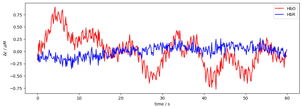
f,ax = p.subplots(1,1, figsize=(12,4))
ax.plot( conc.time, conc.sel(channel="S1D1", chromo="HbO").pint.to("micromolar"), "r-", label="HbO")
ax.plot( conc.time, conc.sel(channel="S1D1", chromo="HbR").pint.to("micromolar"), "b-", label="HbR")
p.legend()
ax.set_xlabel("time / s")
ax.set_ylabel("$\Delta c$ / $\mu M$");