The Recording Container: Cedalion’s main data structure and a guide to indexing
This example notebook introduces the main data classes used by cedalion, and provides examples of how to access and index them.
Overview
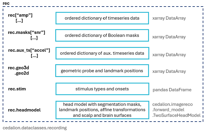
The class ``cedalion.dataclasses.Recording`` is Cedalion’s main data container that can be used to carry related data objects through the program. It can store time series, masks, auxiliary timeseries, probe, headmodel and stimulus information as well as meta data about the recording. It has the following properties:
It resembles the NIRS group in the snirf specification, which provides storage for much of the data stored in a
Recording(e.g. time series map to data elements, probe, stimulus and meta data are stored per NIRS element, etc). Consequently, the methodscedalion.io.read_snirfandcedalion.io.write_snirfmethods operate on lists of recordings.different time series and masks are stored in ordered dictionaries
the user differentiates time series by name
there is a set of canonical names used by
read_snirfto assign names to time seriesCANONICAL_NAMES = { "unprocessed raw": "amp", "processed raw": "amp", "processed dOD": "od", "processed concentrations": "conc", "processed central moments": "moments", "processed blood flow index": "bfi", "processed HRF dOD": "hrf_od", "processed HRF central moments": "hrf_moments", "processed HRF concentrations": "hrf_conc", "processed HRF blood flow index": "hrf_bfi", "processed absorption coefficient": "mua", "processed scattering coefficient": "musp", }
time series are stored in the dictionaries in the order that they were added
convenient access to the last changed time series + canonical names -> consecutive transformations of time series without the need to specify time series by name -> workflows
rec[key]is a shortcut forrec.timeseries[key]not all information stored in a
Recordingcan be stored in snirf files, e.g. for masks, the headmodel and auxiliar objects there is no provision in the snirf specification. We will probably use sidecard files or sidecar hdf groups to store these.
What this notebook covers
This notebook is structured in two parts:
Exploring the ``Recording`` container — how to access timeseries, geometry, stimulus events, quality masks, and the head model.
xarray indexing — how to select data by label, by condition, by time window, or via coordinates of another array. This is the most commonly needed xarray skill for fNIRS analysis.
If you are new to xarray, also have a look at the official xarray indexing documentation.
[1]:
# This cells setups the environment when executed in Google Colab.
try:
    import google.colab
    !curl -s https://raw.githubusercontent.com/ibs-lab/cedalion/dev/scripts/colab_setup.py -o colab_setup.py
    # Select branch with --branch "branch name" (default is "dev")
    %run colab_setup.py
except ImportError:
    pass
Exploring the recording container fields with some example data
[2]:
import os
import cedalion
import cedalion.io
import cedalion.data
import cedalion.xrutils as xrutils
import xarray as xr

# Loading an example dataset will create a recording container.
# Alternatively you can load your ow snirf file using cedalion.io.snirf.read_snirf(PATH_TO_FILE)
rec = cedalion.data.get_fingertapping()
display(rec)
<Recording | timeseries: ['amp'], masks: [], stim: ['1.0', '15.0', '2.0', '3.0'], aux_ts: [], aux_obj: []>
The timeseries field
we loaded raw amplitude data and can now access it:
[3]:
display(rec["amp"])
<xarray.DataArray (channel: 28, wavelength: 2, time: 23239)> Size: 10MB
<Quantity([[[0.0913686 0.0909875 0.0910225 ... 0.0941083 0.0940129 0.0944882]
  [0.1856806 0.186377  0.1836514 ... 0.1856486 0.1850836 0.1842172]]

 [[0.227516  0.2297024 0.2261366 ... 0.2264519 0.2271665 0.226713 ]
  [0.6354927 0.637668  0.6298023 ... 0.6072068 0.6087293 0.6091066]]

 [[0.1064704 0.1066212 0.1053444 ... 0.121114  0.1205022 0.1205441]
  [0.2755033 0.2761615 0.2727006 ... 0.2911952 0.2900544 0.2909847]]

 ...

 [[0.2027881 0.1996586 0.2004866 ... 0.2318743 0.2311941 0.2330808]
  [0.4666358 0.4554404 0.4561614 ... 0.4809749 0.4812827 0.4862896]]

 [[0.4885007 0.4802285 0.4818338 ... 0.6109142 0.6108118 0.613845 ]
  [0.8457658 0.825988  0.8259648 ... 0.975894  0.9756599 0.9826459]]

 [[0.6304559 0.6284427 0.6287045 ... 0.6810626 0.6809573 0.6818709]
  [1.2285622 1.2205907 1.2190002 ... 1.2729124 1.2727222 1.2755645]]], 'volt')>
Coordinates:
  * time        (time) float64 186kB 0.0 0.128 0.256 ... 2.974e+03 2.974e+03
    samples     (time) int64 186kB 0 1 2 3 4 5 ... 23234 23235 23236 23237 23238
  * channel     (channel) object 224B 'S1D1' 'S1D2' 'S1D3' ... 'S8D8' 'S8D16'
    source      (channel) object 224B 'S1' 'S1' 'S1' 'S1' ... 'S8' 'S8' 'S8'
    detector    (channel) object 224B 'D1' 'D2' 'D3' 'D9' ... 'D7' 'D8' 'D16'
  * wavelength  (wavelength) float64 16B 760.0 850.0
Attributes:
data_type_group: unprocessed rawSince we are interested not only in raw “amp”litude data, we convert this data to concentration using the modified beer-lambert law and save it under “conc” in the recording container
[4]:
import cedalion.nirs
# define DPFs and convert to HbO/HbR using the beer lambert law law
dpf = xr.DataArray(
[6, 6],
dims="wavelength",
coords={"wavelength": rec["amp"].wavelength},
)
rec["conc"] = cedalion.nirs.cw.beer_lambert(rec["amp"], rec.geo3d, dpf)
display(rec["conc"])
<xarray.DataArray 'concentration' (chromo: 2, channel: 28, time: 23239)> Size: 10MB
<Quantity([[[ 0.13358239 0.00383028 0.3485663 ... 0.44265804 0.50268758
0.66329562]
[-0.78392182 -0.76400628 -0.63723215 ... 0.23076741 0.20512673
0.16981312]
[ 0.11212379 0.07313248 0.23388668 ... 0.15960301 0.19659632
0.1288759 ]
...
[-0.08996859 0.29760277 0.30354252 ... 0.57096855 0.52735688
0.37714069]
[ 0.90423664 1.3400782 1.38133042 ... -0.27197258 -0.26748648
-0.40128365]
[-0.18579735 0.4272187 0.60694047 ... -0.3055763 -0.29587729
-0.49277044]]
[[ 0.43028905 0.52911229 0.39408018 ... -0.0381295 -0.04878095
-0.16954954]
[ 0.19718417 0.07475109 0.21473068 ... -0.13048136 -0.15862866
-0.12125826]
[ 1.10697449 1.10555197 1.18242296 ... -0.38395394 -0.34006765
-0.31841423]
...
[ 1.13100697 1.16310916 1.11329167 ... -0.65975097 -0.60947889
-0.64605483]
[ 1.82508526 1.8988538 1.83660051 ... -0.85516263 -0.85451739
-0.87311835]
[ 3.67188163 3.63832361 3.54447303 ... -1.07289514 -1.0669728
-1.07564178]]], 'micromolar')>
Coordinates:
* chromo (chromo) <U3 24B 'HbO' 'HbR'
* time (time) float64 186kB 0.0 0.128 0.256 ... 2.974e+03 2.974e+03
samples (time) int64 186kB 0 1 2 3 4 5 ... 23234 23235 23236 23237 23238
* channel (channel) object 224B 'S1D1' 'S1D2' 'S1D3' ... 'S8D8' 'S8D16'
source (channel) object 224B 'S1' 'S1' 'S1' 'S1' ... 'S7' 'S8' 'S8' 'S8'
detector (channel) object 224B 'D1' 'D2' 'D3' 'D9' ... 'D7' 'D8' 'D16'The geo3d field
we have already used channel distances from this field to calculate the concentrations using the beer-lambert law above. The geo3d and geo2d fields are DataArrays of geometric points, whose “magnitude” is the 3d coordinate in 3D / 2D space. They also have two coordinates: a “label”, such as “S1” for Source 1, and a “type” of PointType.Source
[5]:
display(rec.geo3d)
<xarray.DataArray (label: 55, digitized: 3)> Size: 1kB
<Quantity([[-4.16132047e-02 2.67997753e-02 1.29904394e-01]
[-6.47668650e-02 5.81425700e-02 9.08425774e-02]
[-7.12055455e-02 -1.28742727e-02 1.07878609e-01]
[-8.59043654e-02 1.89716985e-02 6.50976243e-02]
[ 3.69417160e-02 2.74838053e-02 1.30221297e-01]
[ 6.06513374e-02 5.88241459e-02 9.11771800e-02]
[ 6.71277139e-02 -1.21992319e-02 1.08572549e-01]
[ 8.18868557e-02 2.04279322e-02 6.57132511e-02]
[-3.76195887e-02 6.32285163e-02 1.15728028e-01]
[-4.13444506e-02 -1.17796113e-02 1.34950029e-01]
[-7.24242465e-02 2.34729321e-02 1.03222190e-01]
[-7.91259275e-02 5.14092912e-02 5.73700461e-02]
[ 3.35271729e-02 6.35996834e-02 1.15838813e-01]
[ 3.68663951e-02 -1.13971649e-02 1.35367241e-01]
[ 6.79159270e-02 2.46825447e-02 1.03666052e-01]
[ 7.53100881e-02 5.22688450e-02 5.78769843e-02]
[-3.77389542e-02 3.40826581e-02 1.29491979e-01]
[-6.14543079e-02 6.44380021e-02 9.06100423e-02]
[-7.28287898e-02 -5.27870528e-03 1.07430548e-01]
[-8.43961064e-02 2.70612338e-02 6.55951074e-02]
...
[-5.79890996e-02 -1.31766082e-02 1.22934918e-01]
[-7.41954904e-02 5.49319712e-03 1.06691588e-01]
[ 2.38285893e-02 3.99629390e-03 1.40819602e-01]
[-8.18419575e-02 2.20987637e-02 8.42248565e-02]
[-8.30909098e-02 3.52083018e-02 6.10323269e-02]
[ 2.64253358e-02 4.33752201e-02 1.29394156e-01]
[ 3.57817707e-02 4.56804970e-02 1.23546335e-01]
[ 3.75562777e-02 8.00119085e-03 1.34555407e-01]
[ 5.40806338e-02 2.67050264e-02 1.18184641e-01]
[ 6.80107631e-02 2.28481808e-02 1.04458720e-01]
[ 4.81712114e-02 6.20348289e-02 1.05182928e-01]
[ 6.46141927e-02 4.23290866e-02 9.77770136e-02]
[ 6.96703241e-02 5.60429038e-02 7.59091889e-02]
[ 7.52694535e-02 3.75789197e-02 8.00743134e-02]
[ 5.28820297e-02 -1.21396142e-02 1.24308118e-01]
[ 6.93801362e-02 6.90166187e-03 1.08064321e-01]
[ 7.93223927e-02 -4.48005459e-04 8.90367069e-02]
[ 7.75602414e-02 2.25155879e-02 8.57843202e-02]
[ 7.91230376e-02 3.64965117e-02 6.25763357e-02]
[ 8.22582105e-02 1.75142331e-02 6.61902835e-02]], 'meter')>
Coordinates:
type (label) object 440B PointType.SOURCE ... PointType.LANDMARK
* label (label) <U3 660B 'S1' 'S2' 'S3' 'S4' 'S5' ... '25' '26' '27' '28'
Dimensions without coordinates: digitizedThe stim field
contains labels for any experimental stimuli that were logged during the recording. Turns out each condition in the experiment was 5 seconds long.
[6]:
display(rec.stim)
| onset | duration | value | trial_type | |
|---|---|---|---|---|
| 0 | 61.824 | 5.0 | 1.0 | 1.0 |
| 1 | 87.296 | 5.0 | 1.0 | 1.0 |
| 2 | 181.504 | 5.0 | 1.0 | 1.0 |
| 3 | 275.712 | 5.0 | 1.0 | 1.0 |
| 4 | 544.640 | 5.0 | 1.0 | 1.0 |
| ... | ... | ... | ... | ... |
| 87 | 2234.112 | 5.0 | 1.0 | 3.0 |
| 88 | 2334.848 | 5.0 | 1.0 | 3.0 |
| 89 | 2362.240 | 5.0 | 1.0 | 3.0 |
| 90 | 2677.504 | 5.0 | 1.0 | 3.0 |
| 91 | 2908.032 | 5.0 | 1.0 | 3.0 |
92 rows × 4 columns
We can see that the trial_type was encoded numerically, which can be hard to read. If we know the experiment we can rename the stimuli using the “rename_events” function
[7]:
rec.stim.cd.rename_events(
{"1.0": "control", "2.0": "Tapping/Left", "3.0": "Tapping/Right"}
)
display(rec.stim)
| onset | duration | value | trial_type | |
|---|---|---|---|---|
| 0 | 61.824 | 5.0 | 1.0 | control |
| 1 | 87.296 | 5.0 | 1.0 | control |
| 2 | 181.504 | 5.0 | 1.0 | control |
| 3 | 275.712 | 5.0 | 1.0 | control |
| 4 | 544.640 | 5.0 | 1.0 | control |
| ... | ... | ... | ... | ... |
| 87 | 2234.112 | 5.0 | 1.0 | Tapping/Right |
| 88 | 2334.848 | 5.0 | 1.0 | Tapping/Right |
| 89 | 2362.240 | 5.0 | 1.0 | Tapping/Right |
| 90 | 2677.504 | 5.0 | 1.0 | Tapping/Right |
| 91 | 2908.032 | 5.0 | 1.0 | Tapping/Right |
92 rows × 4 columns
The masks field
Lastly, we create a mask based on an SNR threshold. A mask is a Boolean DataArray that flags each point across all coordinates as either “true” or “false”, according to the metric applied. Here we use an SNR of 3 to flag all channels in the raw “amp” timeseries as “False” if their SNR is below the threshold. Since SNR is calculated across the whole time, the time dimension gets dropped. Applying this mask later on to a DataArray time series works implitly thanks to the unambiguous xarray coordinates in the mask and timeseries (here for instance the channel name).
[8]:
import cedalion.sigproc.quality as quality
# SNR thresholding using the "snr" function of the quality subpackage using an SNR of 3
_, rec.masks["snr_mask"] = quality.snr(rec["amp"], 3)
display(rec.masks["snr_mask"])
<xarray.DataArray (channel: 28, wavelength: 2)> Size: 56B
array([[ True, True],
[ True, True],
[ True, True],
[ True, True],
[ True, True],
[ True, True],
[ True, True],
[ True, True],
[ True, True],
[ True, True],
[ True, True],
[ True, True],
[ True, True],
[ True, True],
[ True, True],
[ True, True],
[ True, True],
[ True, True],
[ True, True],
[ True, True],
[ True, True],
[ True, True],
[ True, True],
[ True, True],
[ True, True],
[ True, True],
[ True, True],
[ True, True]])
Coordinates:
* channel (channel) object 224B 'S1D1' 'S1D2' 'S1D3' ... 'S8D8' 'S8D16'
source (channel) object 224B 'S1' 'S1' 'S1' 'S1' ... 'S8' 'S8' 'S8'
detector (channel) object 224B 'D1' 'D2' 'D3' 'D9' ... 'D7' 'D8' 'D16'
* wavelength (wavelength) float64 16B 760.0 850.0The headmodel / aux_obj field
The recording container does not yet contain a mask or head model. We load an ICBM152 atlas and create the headmodel
[9]:
import cedalion.dot
rec.head_model = cedalion.dot.get_standard_headmodel("icbm152")
display(rec.head_model)
TwoSurfaceHeadModel(
crs: ijk
tissue_types: csf, gm, scalp, skull, wm
brain faces: 49992 vertices: 25000 units: dimensionless
scalp faces: 20040 vertices: 10018 units: dimensionless
landmarks: 73
)
xarray DataArray Indexing and Selecting Data
xarray DataArrays in Cedalion can be indexed “as usual”. For a complete documentation visit the xarray documentation page. A brief visual overview:
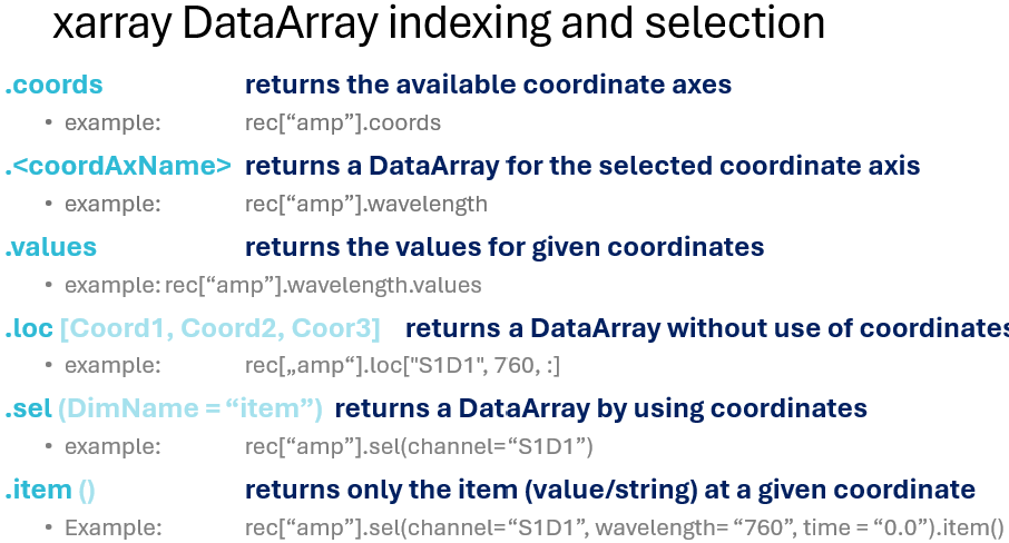
Below we give some examples
[10]:
# first we pull out a time series to save time in the following
ts = rec["amp"]
display(ts)
<xarray.DataArray (channel: 28, wavelength: 2, time: 23239)> Size: 10MB
<Quantity([[[0.0913686 0.0909875 0.0910225 ... 0.0941083 0.0940129 0.0944882]
[0.1856806 0.186377 0.1836514 ... 0.1856486 0.1850836 0.1842172]]
[[0.227516 0.2297024 0.2261366 ... 0.2264519 0.2271665 0.226713 ]
[0.6354927 0.637668 0.6298023 ... 0.6072068 0.6087293 0.6091066]]
[[0.1064704 0.1066212 0.1053444 ... 0.121114 0.1205022 0.1205441]
[0.2755033 0.2761615 0.2727006 ... 0.2911952 0.2900544 0.2909847]]
...
[[0.2027881 0.1996586 0.2004866 ... 0.2318743 0.2311941 0.2330808]
[0.4666358 0.4554404 0.4561614 ... 0.4809749 0.4812827 0.4862896]]
[[0.4885007 0.4802285 0.4818338 ... 0.6109142 0.6108118 0.613845 ]
[0.8457658 0.825988 0.8259648 ... 0.975894 0.9756599 0.9826459]]
[[0.6304559 0.6284427 0.6287045 ... 0.6810626 0.6809573 0.6818709]
[1.2285622 1.2205907 1.2190002 ... 1.2729124 1.2727222 1.2755645]]], 'volt')>
Coordinates:
* time (time) float64 186kB 0.0 0.128 0.256 ... 2.974e+03 2.974e+03
samples (time) int64 186kB 0 1 2 3 4 5 ... 23234 23235 23236 23237 23238
* channel (channel) object 224B 'S1D1' 'S1D2' 'S1D3' ... 'S8D8' 'S8D16'
source (channel) object 224B 'S1' 'S1' 'S1' 'S1' ... 'S8' 'S8' 'S8'
detector (channel) object 224B 'D1' 'D2' 'D3' 'D9' ... 'D7' 'D8' 'D16'
* wavelength (wavelength) float64 16B 760.0 850.0
Attributes:
data_type_group: unprocessed rawit usually helps to know the array’s coordinates. these can be viewed via the .coords xarray accessor. Note that multiple coordinate axes can overlap. For instance, across the time dimension we can use “time” in seconds or “samples” in integer values. Across the “channel” dimension we can index via Source-Detector pairs (e.g. “S1D1”) or via only the “source” or “detector”. The latter will give us all matching elements - e.g. “S1” will give us all channels that contain source S1.
[11]:
display(ts.coords)
Coordinates:
* time (time) float64 186kB 0.0 0.128 0.256 ... 2.974e+03 2.974e+03
samples (time) int64 186kB 0 1 2 3 4 5 ... 23234 23235 23236 23237 23238
* channel (channel) object 224B 'S1D1' 'S1D2' 'S1D3' ... 'S8D8' 'S8D16'
source (channel) object 224B 'S1' 'S1' 'S1' 'S1' ... 'S8' 'S8' 'S8'
detector (channel) object 224B 'D1' 'D2' 'D3' 'D9' ... 'D7' 'D8' 'D16'
* wavelength (wavelength) float64 16B 760.0 850.0
Knowing the coordinates we can also acess the items / labels on the coordinate axes directly
[12]:
display(ts.wavelength) # wavelength dimension
display(ts.time) # time dimension
<xarray.DataArray 'wavelength' (wavelength: 2)> Size: 16B array([760., 850.]) Coordinates: * wavelength (wavelength) float64 16B 760.0 850.0
<xarray.DataArray 'time' (time: 23239)> Size: 186kB
array([0.000000e+00, 1.280000e-01, 2.560000e-01, ..., 2.974208e+03,
       2.974336e+03, 2.974464e+03], shape=(23239,))
Coordinates:
* time (time) float64 186kB 0.0 0.128 0.256 ... 2.974e+03 2.974e+03
samples (time) int64 186kB 0 1 2 3 4 5 ... 23234 23235 23236 23237 23238
Attributes:
units: second… works as expected
[13]:
ts[:,0,:] # first item along wavelength
[13]:
<xarray.DataArray (channel: 28, time: 23239)> Size: 5MB
<Quantity([[0.0913686 0.0909875 0.0910225 ... 0.0941083 0.0940129 0.0944882]
[0.227516 0.2297024 0.2261366 ... 0.2264519 0.2271665 0.226713 ]
[0.1064704 0.1066212 0.1053444 ... 0.121114 0.1205022 0.1205441]
...
[0.2027881 0.1996586 0.2004866 ... 0.2318743 0.2311941 0.2330808]
[0.4885007 0.4802285 0.4818338 ... 0.6109142 0.6108118 0.613845 ]
[0.6304559 0.6284427 0.6287045 ... 0.6810626 0.6809573 0.6818709]], 'volt')>
Coordinates:
* time (time) float64 186kB 0.0 0.128 0.256 ... 2.974e+03 2.974e+03
samples (time) int64 186kB 0 1 2 3 4 5 ... 23234 23235 23236 23237 23238
* channel (channel) object 224B 'S1D1' 'S1D2' 'S1D3' ... 'S8D8' 'S8D16'
source (channel) object 224B 'S1' 'S1' 'S1' 'S1' ... 'S8' 'S8' 'S8'
detector (channel) object 224B 'D1' 'D2' 'D3' 'D9' ... 'D7' 'D8' 'D16'
wavelength float64 8B 760.0
Attributes:
data_type_group: unprocessed raw[14]:
ts[:,:,::3000] # every 3000th time point
[14]:
<xarray.DataArray (channel: 28, wavelength: 2, time: 8)> Size: 4kB
<Quantity([[[0.0913686 0.0907284 0.0909799 0.096484 0.0963254 0.0978755 0.0971495
0.0973881]
[0.1856806 0.1819877 0.180359 0.190375 0.1934964 0.197304 0.1892043
0.1941105]]
[[0.227516 0.2259981 0.2191145 0.2257933 0.2224808 0.224387 0.2252353
0.2337061]
[0.6354927 0.6189633 0.5944316 0.6152465 0.6063239 0.6167434 0.5968902
0.6289392]]
[[0.1064704 0.1106003 0.1113647 0.1181299 0.1185306 0.12127 0.122234
0.1231769]
[0.2755033 0.2795076 0.273957 0.288187 0.2916494 0.3014054 0.2875604
0.3011461]]
[[0.0794062 0.0748053 0.0724615 0.0722422 0.0708733 0.0709404 0.0701675
0.0708531]
[0.128716 0.1205163 0.1162186 0.1156905 0.1142392 0.1144522 0.1130079
0.1140507]]
...
[[0.187484 0.184221 0.1801173 0.179175 0.1779962 0.1764103 0.1753207
0.1750773]
[0.2424386 0.2349307 0.2277864 0.2292719 0.2281034 0.2270149 0.2250216
0.2258399]]
[[0.2027881 0.2103115 0.2106273 0.2227526 0.2268364 0.227802 0.2291271
0.2376249]
[0.4666358 0.4657702 0.4522212 0.4831012 0.4902605 0.5041136 0.4770009
0.5136656]]
[[0.4885007 0.5211291 0.532794 0.5610836 0.5836937 0.5948393 0.5834406
0.5656273]
[0.8457658 0.876043 0.8738404 0.9376701 0.9678892 0.9856668 0.9351691
0.8747212]]
[[0.6304559 0.6529195 0.6589913 0.6675115 0.6719286 0.6761335 0.6776644
0.6881298]
[1.2285622 1.2409274 1.2390135 1.2576277 1.264102 1.2721376 1.269668
1.2924444]]], 'volt')>
Coordinates:
* time (time) float64 64B 0.0 384.0 768.0 ... 2.304e+03 2.688e+03
samples (time) int64 64B 0 3000 6000 9000 12000 15000 18000 21000
* channel (channel) object 224B 'S1D1' 'S1D2' 'S1D3' ... 'S8D8' 'S8D16'
source (channel) object 224B 'S1' 'S1' 'S1' 'S1' ... 'S8' 'S8' 'S8'
detector (channel) object 224B 'D1' 'D2' 'D3' 'D9' ... 'D7' 'D8' 'D16'
* wavelength (wavelength) float64 16B 760.0 850.0
Attributes:
data_type_group: unprocessed rawwithout using the coordinate we require knowledge of the order of dimensions in the DataArray…
[15]:
ts.loc["S1D1", 760, :] # time series for channel S1D1 and wavelength 760nm
[15]:
<xarray.DataArray (time: 23239)> Size: 186kB
<Quantity([0.0913686 0.0909875 0.0910225 ... 0.0941083 0.0940129 0.0944882], 'volt')>
Coordinates:
* time (time) float64 186kB 0.0 0.128 0.256 ... 2.974e+03 2.974e+03
samples (time) int64 186kB 0 1 2 3 4 5 ... 23234 23235 23236 23237 23238
channel <U4 16B 'S1D1'
source object 8B 'S1'
detector object 8B 'D1'
wavelength float64 8B 760.0
Attributes:
data_type_group: unprocessed raw… or we are more explicit, in which case the order does not matter. .sel relies on an index. For some coordinates (time, channel, wavelength) indexes are built. They are printed in bold face when the DataArray is displayed. Indexes are needed for efficient lookup but are not strictly necessary. Hence, we don’t always build them by default.
[16]:
ts.sel(channel="S1D1", wavelength=760) # the same time series as above
[16]:
<xarray.DataArray (time: 23239)> Size: 186kB
<Quantity([0.0913686 0.0909875 0.0910225 ... 0.0941083 0.0940129 0.0944882], 'volt')>
Coordinates:
* time (time) float64 186kB 0.0 0.128 0.256 ... 2.974e+03 2.974e+03
samples (time) int64 186kB 0 1 2 3 4 5 ... 23234 23235 23236 23237 23238
channel <U4 16B 'S1D1'
source object 8B 'S1'
detector object 8B 'D1'
wavelength float64 8B 760.0
Attributes:
data_type_group: unprocessed raw.sel accepts dictionaries. Useful when dimension name is a variable
[17]:
dim = 'wavelength'
dim_value = 760
ts.sel({dim : dim_value})
[17]:
<xarray.DataArray (channel: 28, time: 23239)> Size: 5MB
<Quantity([[0.0913686 0.0909875 0.0910225 ... 0.0941083 0.0940129 0.0944882]
[0.227516 0.2297024 0.2261366 ... 0.2264519 0.2271665 0.226713 ]
[0.1064704 0.1066212 0.1053444 ... 0.121114 0.1205022 0.1205441]
...
[0.2027881 0.1996586 0.2004866 ... 0.2318743 0.2311941 0.2330808]
[0.4885007 0.4802285 0.4818338 ... 0.6109142 0.6108118 0.613845 ]
[0.6304559 0.6284427 0.6287045 ... 0.6810626 0.6809573 0.6818709]], 'volt')>
Coordinates:
* time (time) float64 186kB 0.0 0.128 0.256 ... 2.974e+03 2.974e+03
samples (time) int64 186kB 0 1 2 3 4 5 ... 23234 23235 23236 23237 23238
* channel (channel) object 224B 'S1D1' 'S1D2' 'S1D3' ... 'S8D8' 'S8D16'
source (channel) object 224B 'S1' 'S1' 'S1' 'S1' ... 'S8' 'S8' 'S8'
detector (channel) object 224B 'D1' 'D2' 'D3' 'D9' ... 'D7' 'D8' 'D16'
wavelength float64 8B 760.0
Attributes:
data_type_group: unprocessed rawWe can, for instance, choose only those data points that come after t=10s and before t=60s:
[18]:
ts.sel(time= (ts.time > 10 ) & (ts.time < 60.))
[18]:
<xarray.DataArray (channel: 28, wavelength: 2, time: 390)> Size: 175kB
<Quantity([[[0.0899084 0.0894057 0.0901775 ... 0.0903297 0.090175 0.0899268]
[0.1815226 0.1818538 0.1827682 ... 0.184885 0.1850145 0.1846866]]
[[0.2271194 0.2265271 0.2281751 ... 0.2241381 0.2243378 0.2256896]
[0.6258998 0.6286326 0.6299954 ... 0.6222512 0.6236847 0.627199 ]]
[[0.106186 0.1064838 0.1053833 ... 0.106494 0.1061651 0.1056465]
[0.2714331 0.2728349 0.2736203 ... 0.2736698 0.2742193 0.2759685]]
...
[[0.2022316 0.2017929 0.2027171 ... 0.1998214 0.2007051 0.202647 ]
[0.4570127 0.4581691 0.4631743 ... 0.448159 0.4511331 0.4540838]]
[[0.487628 0.4916749 0.4934949 ... 0.5004812 0.5035935 0.5044765]
[0.8359521 0.8418671 0.8470044 ... 0.8385809 0.8441086 0.8474942]]
[[0.6297619 0.6308818 0.6312802 ... 0.637311 0.6379823 0.6392407]
[1.2148105 1.2171712 1.2189573 ... 1.2232131 1.2258861 1.2278113]]], 'volt')>
Coordinates:
* time (time) float64 3kB 10.11 10.24 10.37 10.5 ... 59.65 59.78 59.9
samples (time) int64 3kB 79 80 81 82 83 84 ... 463 464 465 466 467 468
* channel (channel) object 224B 'S1D1' 'S1D2' 'S1D3' ... 'S8D8' 'S8D16'
source (channel) object 224B 'S1' 'S1' 'S1' 'S1' ... 'S8' 'S8' 'S8'
detector (channel) object 224B 'D1' 'D2' 'D3' 'D9' ... 'D7' 'D8' 'D16'
* wavelength (wavelength) float64 16B 760.0 850.0
Attributes:
data_type_group: unprocessed rawboolean masking works also with the .loc accessor
[19]:
ts.loc[ts.source == "S1"]
[19]:
<xarray.DataArray (channel: 4, wavelength: 2, time: 23239)> Size: 1MB
<Quantity([[[0.0913686 0.0909875 0.0910225 ... 0.0941083 0.0940129 0.0944882]
[0.1856806 0.186377 0.1836514 ... 0.1856486 0.1850836 0.1842172]]
[[0.227516 0.2297024 0.2261366 ... 0.2264519 0.2271665 0.226713 ]
[0.6354927 0.637668 0.6298023 ... 0.6072068 0.6087293 0.6091066]]
[[0.1064704 0.1066212 0.1053444 ... 0.121114 0.1205022 0.1205441]
[0.2755033 0.2761615 0.2727006 ... 0.2911952 0.2900544 0.2909847]]
[[0.0794062 0.0794713 0.0791685 ... 0.0705146 0.0705608 0.0704029]
[0.128716 0.1289733 0.1283794 ... 0.1129772 0.1127544 0.1127884]]], 'volt')>
Coordinates:
* time (time) float64 186kB 0.0 0.128 0.256 ... 2.974e+03 2.974e+03
samples (time) int64 186kB 0 1 2 3 4 5 ... 23234 23235 23236 23237 23238
* channel (channel) object 32B 'S1D1' 'S1D2' 'S1D3' 'S1D9'
source (channel) object 32B 'S1' 'S1' 'S1' 'S1'
detector (channel) object 32B 'D1' 'D2' 'D3' 'D9'
* wavelength (wavelength) float64 16B 760.0 850.0
Attributes:
data_type_group: unprocessed rawfirst via string accessor
[20]:
# regular expression via str accessor
ts.sel(channel=ts.channel.str.match("S[2,3]D[1,2]"))
[20]:
<xarray.DataArray (channel: 4, wavelength: 2, time: 23239)> Size: 1MB
<Quantity([[[0.5512474 0.5510672 0.5476283 ... 0.6179242 0.6188702 0.6187721]
[1.125532 1.1238331 1.1119423 ... 1.1817728 1.1819598 1.1832658]]
[[0.1765604 0.1768194 0.1764903 ... 0.1787845 0.178888 0.1790632]
[0.3228078 0.322831 0.3219485 ... 0.3182213 0.3182161 0.3181564]]
[[0.0577035 0.0581161 0.0575968 ... 0.0606553 0.0603812 0.0608511]
[0.1558412 0.1549238 0.1535897 ... 0.1503445 0.1506066 0.1506666]]
[[0.1679255 0.1679034 0.1677694 ... 0.1610538 0.1611879 0.1610764]
[0.3205449 0.3203354 0.3196127 ... 0.2977933 0.2975577 0.2978071]]], 'volt')>
Coordinates:
* time (time) float64 186kB 0.0 0.128 0.256 ... 2.974e+03 2.974e+03
samples (time) int64 186kB 0 1 2 3 4 5 ... 23234 23235 23236 23237 23238
* channel (channel) object 32B 'S2D1' 'S2D10' 'S3D2' 'S3D11'
source (channel) object 32B 'S2' 'S2' 'S3' 'S3'
detector (channel) object 32B 'D1' 'D10' 'D2' 'D11'
* wavelength (wavelength) float64 16B 760.0 850.0
Attributes:
data_type_group: unprocessed rawor via the use of isin to select a fixed tiem or list of items
[21]:
# item
ts.sel(channel="S1D1")
# list of items
ts.sel(channel=ts.channel.isin(["S1D1", "S8D8"]))
[21]:
<xarray.DataArray (channel: 2, wavelength: 2, time: 23239)> Size: 744kB
<Quantity([[[0.0913686 0.0909875 0.0910225 ... 0.0941083 0.0940129 0.0944882]
[0.1856806 0.186377 0.1836514 ... 0.1856486 0.1850836 0.1842172]]
[[0.4885007 0.4802285 0.4818338 ... 0.6109142 0.6108118 0.613845 ]
[0.8457658 0.825988 0.8259648 ... 0.975894 0.9756599 0.9826459]]], 'volt')>
Coordinates:
* time (time) float64 186kB 0.0 0.128 0.256 ... 2.974e+03 2.974e+03
samples (time) int64 186kB 0 1 2 3 4 5 ... 23234 23235 23236 23237 23238
* channel (channel) object 16B 'S1D1' 'S8D8'
source (channel) object 16B 'S1' 'S8'
detector (channel) object 16B 'D1' 'D8'
* wavelength (wavelength) float64 16B 760.0 850.0
Attributes:
data_type_group: unprocessed rawRepeat: .sel relies on an index. For some coordinates (time, channel, wavelength) indexes are built. They are printed in bold face when the DataArray is displayed. Indexes are needed for efficient lookup but are not strictly necessary. if we would like to index via a coordinate axis for which no index is available (here the “source” coordinate), they can be built:
[22]:
# build the index
ts_with_index = ts.set_xindex("source")
# now we can select by source index
ts_with_index.sel(source="S1")
[22]:
<xarray.DataArray (channel: 4, wavelength: 2, time: 23239)> Size: 1MB
<Quantity([[[0.0913686 0.0909875 0.0910225 ... 0.0941083 0.0940129 0.0944882]
[0.1856806 0.186377 0.1836514 ... 0.1856486 0.1850836 0.1842172]]
[[0.227516 0.2297024 0.2261366 ... 0.2264519 0.2271665 0.226713 ]
[0.6354927 0.637668 0.6298023 ... 0.6072068 0.6087293 0.6091066]]
[[0.1064704 0.1066212 0.1053444 ... 0.121114 0.1205022 0.1205441]
[0.2755033 0.2761615 0.2727006 ... 0.2911952 0.2900544 0.2909847]]
[[0.0794062 0.0794713 0.0791685 ... 0.0705146 0.0705608 0.0704029]
[0.128716 0.1289733 0.1283794 ... 0.1129772 0.1127544 0.1127884]]], 'volt')>
Coordinates:
* time (time) float64 186kB 0.0 0.128 0.256 ... 2.974e+03 2.974e+03
samples (time) int64 186kB 0 1 2 3 4 5 ... 23234 23235 23236 23237 23238
* channel (channel) object 32B 'S1D1' 'S1D2' 'S1D3' 'S1D9'
* source (channel) object 32B 'S1' 'S1' 'S1' 'S1'
detector (channel) object 32B 'D1' 'D2' 'D3' 'D9'
* wavelength (wavelength) float64 16B 760.0 850.0
Attributes:
data_type_group: unprocessed rawHere we use ts.source to select in geo3d values along the ‘label’ dimension. Because ts.source belongs to the ‘channel’ dimension of ts, the resulting xr.DataArray has dimensions ‘channel’ (from ts.source) and ‘digitized’ (from geo3d)
[23]:
display(rec.geo3d)
display(ts.source)
rec.geo3d.loc[ts.source]
<xarray.DataArray (label: 55, digitized: 3)> Size: 1kB
<Quantity([[-4.16132047e-02 2.67997753e-02 1.29904394e-01]
[-6.47668650e-02 5.81425700e-02 9.08425774e-02]
[-7.12055455e-02 -1.28742727e-02 1.07878609e-01]
[-8.59043654e-02 1.89716985e-02 6.50976243e-02]
[ 3.69417160e-02 2.74838053e-02 1.30221297e-01]
[ 6.06513374e-02 5.88241459e-02 9.11771800e-02]
[ 6.71277139e-02 -1.21992319e-02 1.08572549e-01]
[ 8.18868557e-02 2.04279322e-02 6.57132511e-02]
[-3.76195887e-02 6.32285163e-02 1.15728028e-01]
[-4.13444506e-02 -1.17796113e-02 1.34950029e-01]
[-7.24242465e-02 2.34729321e-02 1.03222190e-01]
[-7.91259275e-02 5.14092912e-02 5.73700461e-02]
[ 3.35271729e-02 6.35996834e-02 1.15838813e-01]
[ 3.68663951e-02 -1.13971649e-02 1.35367241e-01]
[ 6.79159270e-02 2.46825447e-02 1.03666052e-01]
[ 7.53100881e-02 5.22688450e-02 5.78769843e-02]
[-3.77389542e-02 3.40826581e-02 1.29491979e-01]
[-6.14543079e-02 6.44380021e-02 9.06100423e-02]
[-7.28287898e-02 -5.27870528e-03 1.07430548e-01]
[-8.43961064e-02 2.70612338e-02 6.55951074e-02]
...
[-5.79890996e-02 -1.31766082e-02 1.22934918e-01]
[-7.41954904e-02 5.49319712e-03 1.06691588e-01]
[ 2.38285893e-02 3.99629390e-03 1.40819602e-01]
[-8.18419575e-02 2.20987637e-02 8.42248565e-02]
[-8.30909098e-02 3.52083018e-02 6.10323269e-02]
[ 2.64253358e-02 4.33752201e-02 1.29394156e-01]
[ 3.57817707e-02 4.56804970e-02 1.23546335e-01]
[ 3.75562777e-02 8.00119085e-03 1.34555407e-01]
[ 5.40806338e-02 2.67050264e-02 1.18184641e-01]
[ 6.80107631e-02 2.28481808e-02 1.04458720e-01]
[ 4.81712114e-02 6.20348289e-02 1.05182928e-01]
[ 6.46141927e-02 4.23290866e-02 9.77770136e-02]
[ 6.96703241e-02 5.60429038e-02 7.59091889e-02]
[ 7.52694535e-02 3.75789197e-02 8.00743134e-02]
[ 5.28820297e-02 -1.21396142e-02 1.24308118e-01]
[ 6.93801362e-02 6.90166187e-03 1.08064321e-01]
[ 7.93223927e-02 -4.48005459e-04 8.90367069e-02]
[ 7.75602414e-02 2.25155879e-02 8.57843202e-02]
[ 7.91230376e-02 3.64965117e-02 6.25763357e-02]
[ 8.22582105e-02 1.75142331e-02 6.61902835e-02]], 'meter')>
Coordinates:
type (label) object 440B PointType.SOURCE ... PointType.LANDMARK
* label (label) <U3 660B 'S1' 'S2' 'S3' 'S4' 'S5' ... '25' '26' '27' '28'
Dimensions without coordinates: digitized<xarray.DataArray 'source' (channel: 28)> Size: 224B
array([np.str_('S1'), np.str_('S1'), np.str_('S1'), np.str_('S1'),
       np.str_('S2'), np.str_('S2'), np.str_('S2'), np.str_('S2'),
       np.str_('S3'), np.str_('S3'), np.str_('S3'), np.str_('S4'),
       np.str_('S4'), np.str_('S4'), np.str_('S5'), np.str_('S5'),
       np.str_('S5'), np.str_('S5'), np.str_('S6'), np.str_('S6'),
       np.str_('S6'), np.str_('S6'), np.str_('S7'), np.str_('S7'),
       np.str_('S7'), np.str_('S8'), np.str_('S8'), np.str_('S8')],
      dtype=object)
Coordinates:
* channel (channel) object 224B 'S1D1' 'S1D2' 'S1D3' ... 'S8D8' 'S8D16'
source (channel) object 224B 'S1' 'S1' 'S1' 'S1' ... 'S7' 'S8' 'S8' 'S8'
detector (channel) object 224B 'D1' 'D2' 'D3' 'D9' ... 'D7' 'D8' 'D16'[23]:
<xarray.DataArray (channel: 28, digitized: 3)> Size: 672B
<Quantity([[-0.0416132   0.02679978  0.12990439]
 [-0.0416132   0.02679978  0.12990439]
 [-0.0416132   0.02679978  0.12990439]
 [-0.0416132   0.02679978  0.12990439]
 [-0.06476686  0.05814257  0.09084258]
 [-0.06476686  0.05814257  0.09084258]
 [-0.06476686  0.05814257  0.09084258]
 [-0.06476686  0.05814257  0.09084258]
 [-0.07120555 -0.01287427  0.10787861]
 [-0.07120555 -0.01287427  0.10787861]
 [-0.07120555 -0.01287427  0.10787861]
 [-0.08590437  0.0189717   0.06509762]
 [-0.08590437  0.0189717   0.06509762]
 [-0.08590437  0.0189717   0.06509762]
 [ 0.03694172  0.02748381  0.1302213 ]
 [ 0.03694172  0.02748381  0.1302213 ]
 [ 0.03694172  0.02748381  0.1302213 ]
 [ 0.03694172  0.02748381  0.1302213 ]
 [ 0.06065134  0.05882415  0.09117718]
 [ 0.06065134  0.05882415  0.09117718]
 [ 0.06065134  0.05882415  0.09117718]
 [ 0.06065134  0.05882415  0.09117718]
 [ 0.06712771 -0.01219923  0.10857255]
 [ 0.06712771 -0.01219923  0.10857255]
 [ 0.06712771 -0.01219923  0.10857255]
 [ 0.08188686  0.02042793  0.06571325]
 [ 0.08188686  0.02042793  0.06571325]
 [ 0.08188686  0.02042793  0.06571325]], 'meter')>
Coordinates:
    type      (channel) object 224B PointType.SOURCE ... PointType.SOURCE
    label     (channel) <U3 336B 'S1' 'S1' 'S1' 'S1' ... 'S7' 'S8' 'S8' 'S8'
  * channel   (channel) object 224B 'S1D1' 'S1D2' 'S1D3' ... 'S8D8' 'S8D16'
    source    (channel) object 224B 'S1' 'S1' 'S1' 'S1' ... 'S7' 'S8' 'S8' 'S8'
    detector  (channel) object 224B 'D1' 'D2' 'D3' 'D9' ... 'D7' 'D8' 'D16'
Dimensions without coordinates: digitizedAccessing xarray DataArray values with .values
e.g. to write them to a numpy array. Example: We want to pull out the actual source names of the first 3 sources..
[24]:
# this way of indexing will not give us what we want, as it returns another xarray with coordinates etc.
display(ts.source[:3])

# instead we use the .values accessors:
display(ts.source.values[:3])
<xarray.DataArray 'source' (channel: 3)> Size: 24B
array([np.str_('S1'), np.str_('S1'), np.str_('S1')], dtype=object)
Coordinates:
  * channel   (channel) object 24B 'S1D1' 'S1D2' 'S1D3'
    source    (channel) object 24B 'S1' 'S1' 'S1'
    detector  (channel) object 24B 'D1' 'D2' 'D3'
array([np.str_('S1'), np.str_('S1'), np.str_('S1')], dtype=object)
Accessing single items in an xarray with .item
indexing a single item in an xarray is still an xarray with coordinates
[25]:
display(ts[0,0,0]) # the first time point of the first channel and first wavelength in the DataArray
<xarray.DataArray ()> Size: 8B
<Quantity(0.0913686, 'volt')>
Coordinates:
    time        float64 8B 0.0
    samples     int64 8B 0
    channel     <U4 16B 'S1D1'
    source      object 8B 'S1'
    detector    object 8B 'D1'
    wavelength  float64 8B 760.0
Attributes:
data_type_group: unprocessed raw[26]:
# to get just the item we use .item()
display(ts[0,0,0].item())
[27]:
# of course this also works with the .sel method
ts.sel(channel="S1D1", wavelength= "760", time = "0.0").item()
[27]:
References
[28]:
cedalion.bib.dump_to_notebook()
Methods used
| [1] | Luke2021 | cedalion.data.get_fingertapping | Robert Luke and David McAlpine. fNIRS Finger Tapping Data in BIDS Format. September 2021. doi:10.5281/zenodo.5529797. |
| [2] | Tucker2022 | cedalion.io.snirf.read_snirf | Stephen Tucker, Jay Dubb, Sreekanth Kura, Alexander von Lühmann, Robert Franke, Jörn M. Horschig, Samuel Powell, Robert Oostenveld, Michael Lührs, Édouard Delaire, Zahra M. Aghajan, Hanseok Yun, Meryem A. Yücel, Qianqian Fang, Theodore J. Huppert, Blaise deB. Frederick, Luca Pollonini, David A. Boas, and Robert Luke. Introduction to the shared near infrared spectroscopy format. Neurophotonics, 10(1):013507, 2022. doi:10.1117/1.NPh.10.1.013507. |
| [3] | Delpy1988 | cedalion.nirs.cw.beer_lambert, cedalion.nirs.cw.int2od, cedalion.nirs.cw.od2conc | D. T. Delpy, M. Cope, P. van der Zee, S. Arridge, S. Wray, and J. Wyatt. Estimation of optical pathlength through tissue from direct time of flight measurement. Physics in Medicine and Biology, 33(12):1433–1442, 1988. doi:10.1088/0031-9155/33/12/008. |
| [4] | Villringer1997 | cedalion.nirs.cw.beer_lambert, cedalion.nirs.cw.int2od, cedalion.nirs.cw.od2conc | Arno Villringer and Britton Chance. Non-invasive optical spectroscopy and imaging of human brain function. Trends in Neurosciences, 20(10):435–442, 1997. doi:10.1016/S0166-2236(97)01132-6. |
| [5] | Prahl1998 | cedalion.nirs.common.get_extinction_coefficients | Scott A. Prahl. Optical absorption of hemoglobin. Oregon Medical Laser Center, online resource, 1998. URL: https://omlc.org/spectra/hemoglobin/. |
| [6] | Huppert2009 | cedalion.sigproc.quality.snr | Theodore J. Huppert, Solomon G. Diamond, Maria A. Franceschini, and David A. Boas. Homer: a review of time-series analysis methods for near-infrared spectroscopy of the brain. Appl. Opt., 48(10):D280–D298, Apr 2009. doi:https://doi.org/10.1364/AO.48.00D280. |
| [7] | Fonov2011 | cedalion.data.get_icbm152_headmodel_files | Vladimir Fonov, Alan C. Evans, Kelly Botteron, C. Robert Almli, Robert C. McKinstry, and D. Louis Collins. Unbiased average age-appropriate atlases for pediatric studies. NeuroImage, 54(1):313–327, January 2011. doi:10.1016/j.neuroimage.2010.07.033. |
| [8] | Fischl2012 | cedalion.data.get_icbm152_headmodel_files | Bruce Fischl. FreeSurfer. NeuroImage, 62(2):774–781, 2012. doi:10.1016/j.neuroimage.2012.01.021. |
| [9] | Schaefer2018 | cedalion.data.get_icbm152_headmodel_files | Alexander Schaefer, Ru Kong, Evan M Gordon, Timothy O Laumann, Xi-Nian Zuo, Avram J Holmes, Simon B Eickhoff, and BT Thomas Yeo. Local-global parcellation of the human cerebral cortex from intrinsic functional connectivity mri. Cerebral cortex, 28(9):3095–3114, 2018. doi:10.1093/cercor/bhx179. |