S7: Data Augmentation
This example notebook illustrates the functionality in cedalion.sim.synthetic_hrf and cedalion.sim.synthetic_artifact to create simulated datasets with added activations and motion artifacts.
It has two parts:
Learning objectives
In this notebook you will learn to:
Generate synthetic HRF-modulated fNIRS signals with controllable parameters
Add realistic motion artefacts to clean recordings
Use augmented data for algorithm benchmarking with known ground truth
[1]:
# This cells setups the environment when executed in Google Colab.
try:
    import google.colab
    !curl -s https://raw.githubusercontent.com/ibs-lab/cedalion/dev/scripts/colab_setup.py -o colab_setup.py
    # Select branch with --branch "branch name" (default is "dev")
    %run colab_setup.py
except ImportError:
    pass
[2]:
# set this flag to True to enable interactive 3D plots
INTERACTIVE_PLOTS = False
[3]:
import matplotlib.pyplot as plt
import numpy as np
import pyvista as pv
import xarray as xr

import cedalion
import cedalion.dataclasses as cdc
import cedalion.data
import cedalion.geometry.landmarks as cd_landmarks
import cedalion.dot as dot
import cedalion.models.glm as glm
import cedalion.nirs

import cedalion.vis.anatomy
import cedalion.vis.blocks as vbx

import cedalion.sigproc.quality as quality
import cedalion.sim.synthetic_hrf as synhrf
import cedalion.sim.synthetic_artifact as synart
import cedalion.xrutils as xrutils
from cedalion import units
from IPython.display import Image

xr.set_options(display_expand_data=False)

if INTERACTIVE_PLOTS:
    pv.set_jupyter_backend('server')
else:
    pv.set_jupyter_backend('static')
[4]:
# helper function to display gifs in rendered notbooks
def display_image(fname : str):
    display(Image(data=open(fname,'rb').read(), format='png'))
Adding Synthetic Activations
Loading and preprocessing the dataset
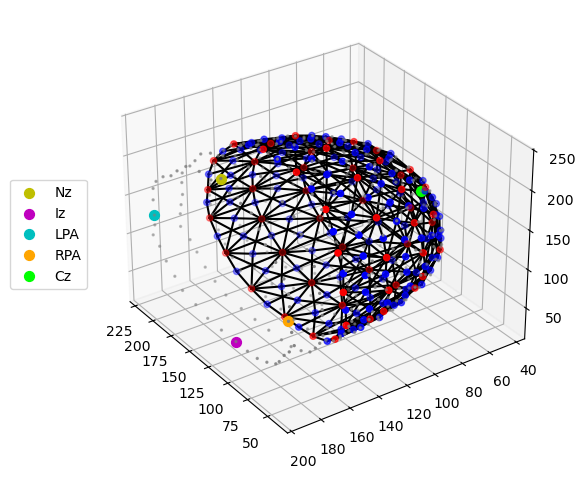
This notebook uses a high-density, whole head resting state dataset recorded with a NinjaNIRS 22.
[5]:
rec = cedalion.data.get_nn22_resting_state()

geo3d = rec.geo3d
meas_list = rec._measurement_lists["amp"]

amp = rec["amp"]
amp = amp.pint.dequantify().pint.quantify("V")

display(amp)
<xarray.DataArray (channel: 567, wavelength: 2, time: 3310)> Size: 30MB
[V] 0.05955 0.0596 0.05969 0.0598 0.05993 ... 0.3148 0.3137 0.3136 0.3136 0.3144
Coordinates:
  * time        (time) float64 26kB 0.0 0.1112 0.2225 ... 367.9 368.0 368.1
    samples     (time) int64 26kB 0 1 2 3 4 5 ... 3304 3305 3306 3307 3308 3309
  * channel     (channel) object 5kB 'S10D87' 'S10D94' ... 'S47D29' 'S5D137'
    source      (channel) object 5kB 'S10' 'S10' 'S10' ... 'S56' 'S47' 'S5'
    detector    (channel) object 5kB 'D87' 'D94' 'D89' ... 'D129' 'D29' 'D137'
  * wavelength  (wavelength) float64 16B 760.0 850.0
Attributes:
data_type_group: unprocessed raw[6]:
cedalion.vis.anatomy.plot_montage3D(rec["amp"], geo3d)
[7]:
# Select channels which have at least a signal-to-noise ratio of 10
snr_thresh = 10  # the SNR (std/mean) of a channel.
snr, snr_mask = quality.snr(rec["amp"], snr_thresh)
amp_selected, masked_channels = xrutils.apply_mask(
    rec["amp"], snr_mask, "drop", "channel"
)

print(f"Removed {len(masked_channels)} channels because of low SNR.")
Removed 23 channels because of low SNR.
[8]:
# Calculate optical density
od = cedalion.nirs.cw.int2od(amp_selected)
Construct headmodel
We load the the Colin27 headmodel, since we need the geometry for image reconstruction.
[9]:
head_ijk = dot.get_standard_headmodel("colin27")

# transform coordinates to a RAS coordinate system
head_ras = head_ijk.apply_transform(head_ijk.t_ijk2ras)
[10]:
display(head_ijk.brain)
display(head_ras.brain)
TrimeshSurface(faces: 49992 vertices: 25000 crs: ijk units: dimensionless vertex_coords: ['fsaverage_vertex', 'parcel', 'mni152_r', 'mni152_a', 'mni152_s'])
TrimeshSurface(faces: 49992 vertices: 25000 crs: mni units: millimeter vertex_coords: ['fsaverage_vertex', 'parcel', 'mni152_r', 'mni152_a', 'mni152_s'])
[11]:
head_ras.landmarks
[11]:
<xarray.DataArray (label: 73, mni: 3)> Size: 2kB
[mm] 0.0045 -118.6 -23.08 -86.08 -19.99 ... -100.4 37.02 49.81 -99.34 21.47
Coordinates:
  * label    (label) <U3 876B 'Iz' 'LPA' 'RPA' 'Nz' ... 'PO1' 'PO2' 'PO4' 'PO6'
    type     (label) object 584B PointType.LANDMARK ... PointType.LANDMARK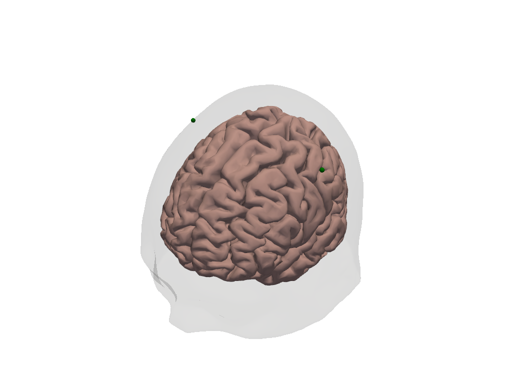
Dimensions without coordinates: mniWe want to build the synthetic HRFs at C3 and C4 (green dots in the image below)
[12]:
plt_pv = pv.Plotter()
vbx.plot_surface(plt_pv, head_ras.brain, color="#d3a6a1")
vbx.plot_surface(plt_pv, head_ras.scalp, opacity=0.1)
vbx.plot_labeled_points(
    plt_pv, head_ras.landmarks.sel(label=["C3", "C4"]), show_labels=True
)
vbx.camera_at_cog(plt_pv, head_ras.brain, (-400,500,400), fit_scene=True)

plt_pv.show()
Build spatial activation pattern on brain surface for landmarks C3 and C4
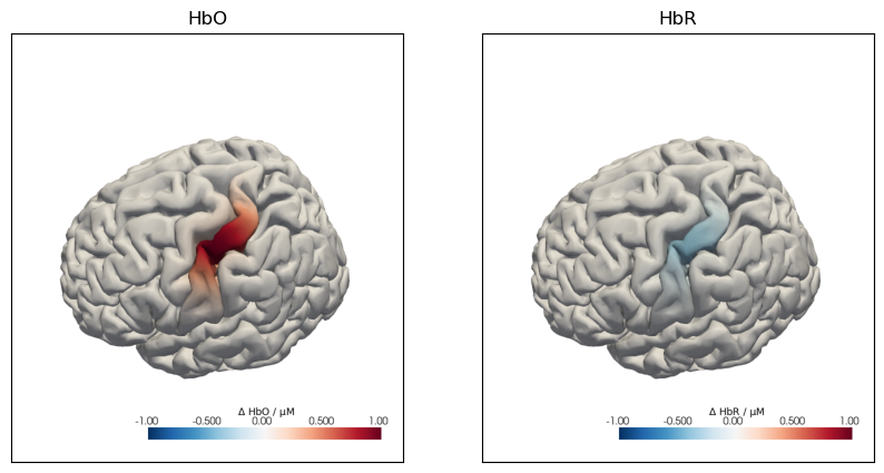
The function build_spatial_activation is used to place a spatial activation pattern on the brain surface. The activation pattern is a Gaussian function of the geodesic distance to a seed vertex. Hence, the size of the activation is determined by the standard deviation of this Gaussian, specified by the parameter spatial_scale. The peak intensity in HbO is determined by the parameter intensity_scale. The intensity of HbR activation is specified relative to the HbO peak intensity. So
if the HbO pattern describes an increase in Hbo then providing a negative factor smaller than 1 yields a decrease in HbR with smaller amplitude. The seed vertex (integer) can be selected as the closest vertex to a given landmark:
[13]:
# obtain the closest vertices to C3 and C4
_, c3_seed = head_ras.brain.mesh.kdtree.query(
    head_ras.landmarks.sel(label="C3").pint.magnitude
)
_, c4_seed = head_ras.brain.mesh.kdtree.query(
    head_ras.landmarks.sel(label="C4").pint.magnitude
)
[14]:
# create the spatial activation
spatial_act = synhrf.build_spatial_activation(
    head_ras.brain,
    c3_seed,
    spatial_scale=2 * cedalion.units.cm,
    intensity_scale=1 * units.micromolar,
    hbr_scale=-0.4,
)
The resulting DataArray contains an activation value for each vertex and chromophore on the brain surface.
[15]:
display(spatial_act)
<xarray.DataArray (vertex: 25000, chromo: 2)> Size: 400kB
[M] 1.303e-29 -5.211e-30 3.318e-30 -1.327e-30 9.361e-31 ... 0.0 -0.0 0.0 -0.0
Coordinates:
  * chromo   (chromo) <U3 24B 'HbO' 'HbR'
Dimensions without coordinates: vertex
[16]:
f,ax = plt.subplots(1,2,figsize=(10,5))
cedalion.vis.anatomy.plot_brain_in_axes(
        od,
        head_ras.landmarks,
        spatial_act.sel(chromo="HbO").pint.to("uM"),
        head_ras.brain,
        ax[0],
        camera_pos="C3",
        cmap="RdBu_r",
        vmin=-1,
        vmax=+1,
        cb_label=r"$\Delta$ HbO / µM",
        title=None,
    )
ax[0].set_title("HbO")
cedalion.vis.anatomy.plot_brain_in_axes(
        od,
        head_ras.landmarks,
        spatial_act.sel(chromo="HbR").pint.to("uM"),
        head_ras.brain,
        ax[1],
        camera_pos="C3",
        cmap="RdBu_r",
        vmin=-1,
        vmax=+1,
        cb_label=r"$\Delta$ HbR / µM",
        title=None,
    )
ax[1].set_title("HbR");
The following plot illustrates the effects of the spatial_scale and intensity_scale parameters:
[17]:
f, ax = plt.subplots(2, 3, figsize=(9, 6))
for i, spatial_scale in enumerate([0.5 * units.cm, 2 * units.cm, 3 * units.cm]):
    spatial_act = synhrf.build_spatial_activation(
        head_ras.brain,
        c3_seed,
        spatial_scale=spatial_scale,
        intensity_scale=1 * units.micromolar,
        hbr_scale=-0.4,
    )

    cedalion.vis.anatomy.plot_brain_in_axes(
        od,
        head_ras.landmarks,
        spatial_act.sel(chromo="HbO").pint.to("uM"),
        head_ras.brain,
        ax[0, i],
        camera_pos="C3",
        cmap="RdBu_r",
        vmin=-1,
        vmax=+1,
        cb_label=r"$\Delta$ HbO / µM",
        title=None,
    )
    ax[0, i].set_title(f"spatial_scale: {spatial_scale.magnitude} cm")

for i, intensity_scale in enumerate(
    [
        0.5 * units.micromolar,
        1.0 * units.micromolar,
        2.0 * units.micromolar,
    ]
):
    spatial_act = synhrf.build_spatial_activation(
        head_ras.brain,
        c3_seed,
        spatial_scale=2 * units.cm,
        intensity_scale=intensity_scale,
        hbr_scale=-0.4,
    )

    cedalion.vis.anatomy.plot_brain_in_axes(
        od,
        head_ras.landmarks,
        spatial_act.sel(chromo="HbO").pint.to("uM"),
        head_ras.brain,
        ax[1, i],
        camera_pos="C3",
        cmap="RdBu_r",
        vmin=-2,
        vmax=+2,
        cb_label=r"$\Delta$ HbO / µM",
        title=None,
    )
    ax[1, i].set_title(f"intensity_scale: {intensity_scale.magnitude} µM")

f.tight_layout()
For this example notebook two activations are placed below C3 and C4:
[18]:
spatial_act_c3 = synhrf.build_spatial_activation(
    head_ras.brain,
    c3_seed,
    spatial_scale=2 * cedalion.units.cm,
    intensity_scale=1 * units.micromolar,
    hbr_scale=-0.4,
)
spatial_act_c4 = synhrf.build_spatial_activation(
    head_ras.brain,
    c4_seed,
    spatial_scale=2 * cedalion.units.cm,
    intensity_scale=1 * units.micromolar,
    hbr_scale=-0.4,
)
We concatenate the two images for C3 and C4 along dimension trial_type to get a single DataArray with the spatial information for both landmarks.
[19]:
# concatenate the two spatial activations along a new dimension
spatial_imgs = xr.concat(
    [spatial_act_c3, spatial_act_c4], dim="trial_type"
).assign_coords(trial_type=["Stim C3", "Stim C4"])
spatial_imgs
[19]:
<xarray.DataArray (trial_type: 2, vertex: 25000, chromo: 2)> Size: 800kB
[M] 1.303e-29 -5.211e-30 3.318e-30 ... -3.621e-22 7.069e-35 -2.828e-35
Coordinates:
  * chromo      (chromo) <U3 24B 'HbO' 'HbR'
  * trial_type  (trial_type) <U7 56B 'Stim C3' 'Stim C4'
Dimensions without coordinates: vertex
Plots of spatial patterns
Using the helper function cedalion.vis.anatomy.plot_brain_in_axes, the created activations on the brain surface below C3 and C4 are plotted:
[20]:
f, ax = plt.subplots(1,2, figsize=(10,5))

cedalion.vis.anatomy.plot_brain_in_axes(
    od,
    head_ras.landmarks,
    spatial_imgs.sel(trial_type="Stim C3", chromo="HbO").pint.to("uM"),
    head_ras.brain,
    ax[0],
    camera_pos="C3",
    cmap="RdBu_r",
    vmin=-1,
    vmax=+1,
    cb_label=r"$\Delta$ HbO / µM",
    title="C3 Activation",
)

cedalion.vis.anatomy.plot_brain_in_axes(
    od,
    head_ras.landmarks,
    spatial_imgs.sel(trial_type="Stim C4", chromo="HbO").pint.to("uM"),
    head_ras.brain,
    ax[1],
    camera_pos="C4",
    cmap="RdBu_r",
    vmin=-1,
    vmax=+1,
    cb_label=r"$\Delta$ HbO / µM",
    title="C4 Activation",
)

f.tight_layout()
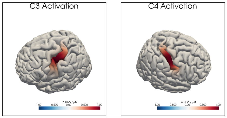
Image Reconstruction
We load the precomputed Adot matrix to be able to map from image to channel space. (For details see S5 image reconstruction tutorial).
[21]:
Adot = cedalion.data.get_precomputed_sensitivity("nn22_resting", "colin27")
[22]:
# we only consider brain vertices, not scalp and drop pruned channels
Adot_brain = Adot.sel(vertex=Adot.is_brain, channel=od.channel)
Adot_brain
[22]:
<xarray.DataArray (channel: 544, vertex: 25000, wavelength: 2)> Size: 109MB
1.038e-18 1.038e-18 2.69e-18 2.69e-18 ... 5.42e-13 5.42e-13 1.069e-22 1.069e-22
Coordinates:
    parcel      (vertex) object 200kB 'VisCent_ExStr_8_LH' ... 'VisCent_ExStr...
    is_brain    (vertex) bool 25kB True True True True ... True True True True
  * channel     (channel) object 4kB 'S10D87' 'S10D94' ... 'S47D29' 'S5D137'
    detector    (channel) object 4kB 'D87' 'D94' 'D89' ... 'D129' 'D29' 'D137'
    source      (channel) object 4kB 'S10' 'S10' 'S10' ... 'S56' 'S47' 'S5'
  * wavelength  (wavelength) float64 16B 760.0 850.0
Dimensions without coordinates: vertex
Attributes:
units: mmThe forward model and image reconstruction transform time series in image space into channel space, and vice versa. In the present case, we need to translate between optical-density time series of different wavelengths in channel space and concentration time series of different chromophores in image space. This is facilitated by the function dot.forward_model.image_to_channel_space:
[23]:
# propagate concentration changes in the brain to optical density
# changes in channel space

spatial_chan = dot.forward_model.image_to_channel_space(
    Adot_brain, spatial_imgs, spectrum="prahl"
)
spatial_chan
[23]:
<xarray.DataArray (trial_type: 2, wavelength: 2, channel: 544)> Size: 17kB
[] -6.863e-13 -1.992e-11 -1.644e-11 -5.69e-14 ... 1.434e-06 2.526e-08 2.487e-08
Coordinates:
  * wavelength  (wavelength) float64 16B 760.0 850.0
  * channel     (channel) object 4kB 'S10D112' 'S10D133' ... 'S9D94' 'S9D96'
  * trial_type  (trial_type) <U7 56B 'Stim C3' 'Stim C4'
    source      (channel) object 4kB 'S10' 'S10' 'S10' 'S10' ... 'S9' 'S9' 'S9'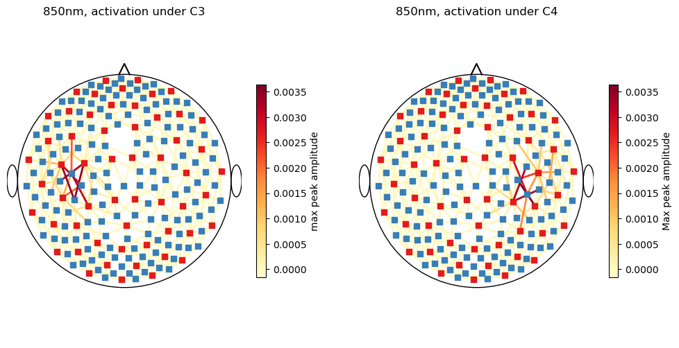
detector (channel) object 4kB 'D112' 'D133' 'D135' ... 'D92' 'D94' 'D96'Show the spatial activation in channel space with a scalp plot.
[24]:
fig, ax = plt.subplots(1, 2)
# adjust plot size
fig.set_size_inches(12, 6)
cedalion.vis.anatomy.scalp_plot(
    od,
    rec.geo3d,
    spatial_chan.sel(trial_type="Stim C3", wavelength=850),
    ax[0],
    cmap="YlOrRd",
    title="850nm, activation under C3",
    vmin=spatial_chan.min().item(),
    vmax=spatial_chan.max().item(),
    cb_label="max peak amplitude",
)
cedalion.vis.anatomy.scalp_plot(
    od,
    rec.geo3d,
    spatial_chan.sel(trial_type="Stim C4", wavelength=850),
    ax[1],
    cmap="YlOrRd",
    title="850nm, activation under C4",
    vmin=spatial_chan.min().item(),
    vmax=spatial_chan.max().item(),
    cb_label="Max peak amplitude",
)
plt.show()
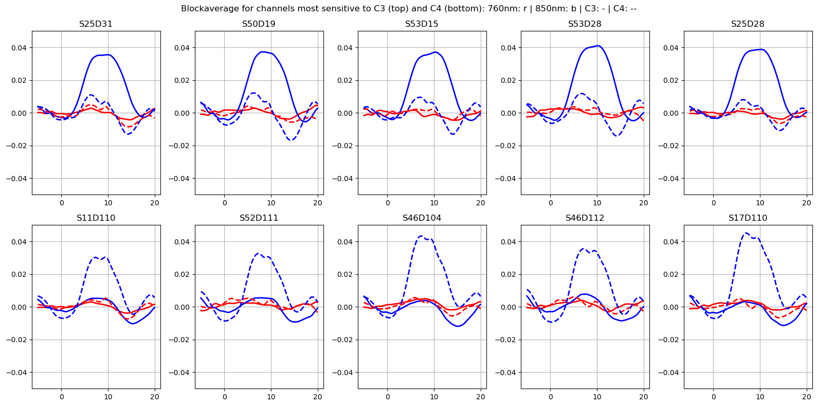
Get top 5 channels for each trial type where synthetic activation is highest
[25]:
roi_chans_c3 = spatial_chan.channel[
    spatial_chan.sel(trial_type="Stim C3").max("wavelength").argsort()[-5:].values
].values
roi_chans_c4 = spatial_chan.channel[
    spatial_chan.sel(trial_type="Stim C4").max("wavelength").argsort()[-5:].values
].values
Concentration Scale
The activations were simulataed in image space with a peak concentration change of 1 µM in one vertex. The change in optical density in one channel reflects concentration changes in the ensemble of vertices that this channel is sensitive to.
When applying the Beer-Lambert-transformation in channel space, a change in concentration is calculated for each channel. However, the scales of these concentration changes and the concentration changes in single vertices are not the same.
Here, a correction factor is calculated to scale the activation in channel space to 1uM.
[26]:
dpf = xr.DataArray(
    [6, 6],
    dims="wavelength",
    coords={"wavelength": rec["amp"].wavelength},
)

# add time axis with one time point so we can convert to conc
spatial_chan_w_time = spatial_chan.expand_dims("time")
spatial_chan_w_time = spatial_chan_w_time.assign_coords(time=[0])
spatial_chan_w_time.time.attrs["units"] = "second"
display(spatial_chan_w_time)
spatial_chan_conc = cedalion.nirs.cw.od2conc(
    spatial_chan_w_time, geo3d, dpf, spectrum="prahl"
)
<xarray.DataArray (time: 1, trial_type: 2, wavelength: 2, channel: 544)> Size: 17kB
[] -6.863e-13 -1.992e-11 -1.644e-11 -5.69e-14 ... 1.434e-06 2.526e-08 2.487e-08
Coordinates:
  * wavelength  (wavelength) float64 16B 760.0 850.0
  * channel     (channel) object 4kB 'S10D112' 'S10D133' ... 'S9D94' 'S9D96'
  * trial_type  (trial_type) <U7 56B 'Stim C3' 'Stim C4'
    source      (channel) object 4kB 'S10' 'S10' 'S10' 'S10' ... 'S9' 'S9' 'S9'
    detector    (channel) object 4kB 'D112' 'D133' 'D135' ... 'D92' 'D94' 'D96'
* time (time) int64 8B 0[27]:
# rescale so that synthetic hrfs add 1 micromolar at peak.
rescale_factor = (1* units.micromolar / spatial_chan_conc.max()).item()

display(rescale_factor)
spatial_chan *= rescale_factor
HRFs in channel space
So far the notebook focused on the spatial extent of the activation. To build the temporal HRF model we use the same functionality that generates hrf regressors for the GLM.
First we select a basis function, which defines the temporal shape of the HRF.
[28]:
basis_fct = glm.Gamma(tau=0 * units.s, sigma=3 * units.s, T=3 * units.s)
[29]:
od.time
[29]:
<xarray.DataArray 'time' (time: 3310)> Size: 26kB
0.0 0.1112 0.2225 0.3337 0.445 0.5562 ... 367.6 367.7 367.8 367.9 368.0 368.1
Coordinates:
  * time     (time) float64 26kB 0.0 0.1112 0.2225 0.3337 ... 367.9 368.0 368.1
    samples  (time) int64 26kB 0 1 2 3 4 5 6 ... 3304 3305 3306 3307 3308 3309
Attributes:
units: secondA Stim DataFrame, which contains the onset, duration and amplitude of the synthetic HRFs, is created.
[30]:
stim_df = synhrf.build_stim_df(
    max_time=od.time.values[-1] * units.seconds,
    trial_types=["Stim C3", "Stim C4"],
    min_interval=10 * units.seconds,
    max_interval=20 * units.seconds,
    min_stim_dur = 10 * units.seconds,
    max_stim_dur = 10 * units.seconds,
    min_stim_value = 1.0,
    max_stim_value = 1.0,
    order="random",
)
[31]:
stim_df.head()
[31]:
| onset | duration | value | trial_type | |
|---|---|---|---|---|
| 0 | 17.84 | 10.0 | 1.0 | Stim C4 |
| 1 | 42.27 | 10.0 | 1.0 | Stim C4 |
| 2 | 70.29 | 10.0 | 1.0 | Stim C4 |
| 3 | 91.77 | 10.0 | 1.0 | Stim C3 |
| 4 | 121.44 | 10.0 | 1.0 | Stim C3 |
We can now use our stim dataframe, basis function, and spatial information to create the synthetic HRF timeseries
[32]:
syn_ts = synhrf.build_synthetic_hrf_timeseries(od, stim_df, basis_fct, spatial_chan)
We get a synthetic HRF timeseries for each channel, trial_type and chromo / wavelength
[33]:
syn_ts
[33]:
<xarray.DataArray (trial_type: 2, wavelength: 2, channel: 544, time: 3310)> Size: 58MB
[] -0.0 -0.0 -0.0 -0.0 -0.0 -0.0 -0.0 -0.0 ... 0.0 0.0 0.0 0.0 0.0 0.0 0.0 0.0
Coordinates:
  * wavelength  (wavelength) float64 16B 760.0 850.0
  * channel     (channel) object 4kB 'S10D112' 'S10D133' ... 'S9D94' 'S9D96'
  * trial_type  (trial_type) <U7 56B 'Stim C3' 'Stim C4'
    source      (channel) object 4kB 'S10' 'S10' 'S10' 'S10' ... 'S9' 'S9' 'S9'
    detector    (channel) object 4kB 'D112' 'D133' 'D135' ... 'D92' 'D94' 'D96'
* time (time) float64 26kB 0.0 0.1112 0.2225 ... 367.9 368.0 368.1Sum the synthetic timeseries over trial_type dimension, so it has the same shape as the resting state data
[34]:
syn_ts_sum = syn_ts.sum(dim='trial_type')
syn_ts_sum
[34]:
<xarray.DataArray (wavelength: 2, channel: 544, time: 3310)> Size: 29MB
[] 0.0 0.0 0.0 0.0 0.0 0.0 0.0 0.0 0.0 ... 0.0 0.0 0.0 0.0 0.0 0.0 0.0 0.0 0.0
Coordinates:
  * wavelength  (wavelength) float64 16B 760.0 850.0
  * channel     (channel) object 4kB 'S10D112' 'S10D133' ... 'S9D94' 'S9D96'
    source      (channel) object 4kB 'S10' 'S10' 'S10' 'S10' ... 'S9' 'S9' 'S9'
    detector    (channel) object 4kB 'D112' 'D133' 'D135' ... 'D92' 'D94' 'D96'
* time (time) float64 26kB 0.0 0.1112 0.2225 ... 367.9 368.0 368.1Adding HRFs to measured data
Here, the simulated activations are combined with physiological noise by adding the synthetic HRFs to the resting state dataset:
[35]:
# set to false to process only the synth. HRF in the following
ADD_RESTING_STATE = True

if ADD_RESTING_STATE:
    od_w_hrf = od + syn_ts_sum
else:
    od_w_hrf = syn_ts_sum
    od_w_hrf = od_w_hrf.assign_coords(
        {
            "samples": ("time", od.samples.values),
            "time": ("time", od.time.data),
        }
    )
    od_w_hrf = od_w_hrf.pint.quantify({"time": "s"})
Recover the HRFs again
In the following, the added activations should be extracted from the simulated dataset again. To this end, the data is frequency filtered and block averages are calculated.
[36]:
od_w_hrf_filtered = od_w_hrf.cd.freq_filter(fmin=0.02, fmax=0.5, butter_order=4)
[37]:
od_w_hrf_filtered
[37]:
<xarray.DataArray (channel: 544, wavelength: 2, time: 3310)> Size: 29MB
[] -0.001577 -0.00252 -0.003411 -0.004201 ... 0.0001448 0.0007453 0.001379
Coordinates:
  * time        (time) float64 26kB 0.0 0.1112 0.2225 ... 367.9 368.0 368.1
  * channel     (channel) object 4kB 'S10D87' 'S10D94' ... 'S47D29' 'S5D137'
  * wavelength  (wavelength) float64 16B 760.0 850.0
    samples     (time) int64 26kB 0 1 2 3 4 5 ... 3304 3305 3306 3307 3308 3309
    source      (channel) object 4kB 'S10' 'S10' 'S10' ... 'S56' 'S47' 'S5'
detector (channel) object 4kB 'D87' 'D94' 'D89' ... 'D129' 'D29' 'D137'[38]:
epochs = od_w_hrf_filtered.cd.to_epochs(
    stim_df,  # stimulus dataframe
    ["Stim C3", "Stim C4"],  # select events
    before=5 * units.seconds,  # seconds before stimulus
    after=20 * units.seconds,  # seconds after stimulus
)

# calculate baseline
baseline = epochs.sel(reltime=(epochs.reltime < 0)).mean("reltime")
# subtract baseline
epochs_blcorrected = epochs - baseline

# group trials by trial_type. For each group individually average the epoch dimension
blockaverage = epochs_blcorrected.groupby("trial_type").mean("epoch")

n_roi = roi_chans_c3.size
# show results
f, ax = plt.subplots(2, n_roi, figsize=(16, 8))
ax = ax.flatten()
for i_ch, ch in enumerate(roi_chans_c3):
    for ls, trial_type in zip(["-", "--"], blockaverage.trial_type):
        ax[i_ch].plot(
            blockaverage.reltime,
            blockaverage.sel(wavelength=760, trial_type=trial_type, channel=ch),
            "r",
            lw=2,
            ls=ls,
        )
        ax[i_ch].plot(
            blockaverage.reltime,
            blockaverage.sel(wavelength=850, trial_type=trial_type, channel=ch),
            "b",
            lw=2,
            ls=ls,
        )
    ax[i_ch].grid(1)
    ax[i_ch].set_title(ch)
    ax[i_ch].set_ylim(-0.05, 0.05)

for i_ch, ch in enumerate(roi_chans_c4):
    for ls, trial_type in zip(["-", "--"], blockaverage.trial_type):
        ax[i_ch + n_roi].plot(
            blockaverage.reltime,
            blockaverage.sel(wavelength=760, trial_type=trial_type, channel=ch),
            "r",
            lw=2,
            ls=ls,
        )
        ax[i_ch + n_roi].plot(
            blockaverage.reltime,
            blockaverage.sel(wavelength=850, trial_type=trial_type, channel=ch),
            "b",
            lw=2,
            ls=ls,
        )
    ax[i_ch + n_roi].grid(1)
    ax[i_ch + n_roi].set_title(ch)
    ax[i_ch + n_roi].set_ylim(-0.05, 0.05)

plt.suptitle(
    "Blockaverage for channels most sensitive to C3 (top) and C4 (bottom): 760nm: r | 850nm: b | C3: - | C4: --"
)
plt.tight_layout()
plt.show()
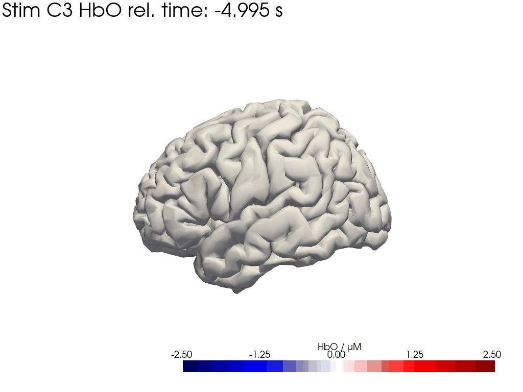
Map block average back to brain surface
We map our extracted block averages back to the brain surface to visualize the recovered HRFs activation for Stim C3. We can compare it to the synthetic HRF image we created earlier.
[39]:
recon = dot.ImageRecon(
    Adot,
    recon_mode="mua2conc",
    alpha_meas=0.5,
    brain_only=True,
    spatial_basis_functions=None
)

blockaverage_img = recon.reconstruct(blockaverage)
blockaverage_img
[39]:
<xarray.DataArray (chromo: 2, vertex: 25000, trial_type: 2, reltime: 226)> Size: 181MB
[µM] -0.02184 -0.01854 -0.01389 -0.008007 ... -0.0004502 -0.0003955 -0.0003436
Coordinates:
  * chromo      (chromo) <U3 24B 'HbO' 'HbR'
    parcel      (vertex) object 200kB 'VisCent_ExStr_8_LH' ... 'VisCent_ExStr...
    is_brain    (vertex) bool 25kB True True True True ... True True True True
  * reltime     (reltime) float64 2kB -4.995 -4.884 -4.773 ... 19.76 19.87 19.98
  * trial_type  (trial_type) object 16B 'Stim C3' 'Stim C4'
Dimensions without coordinates: vertex[40]:
# plot HbO time trace of left and right brain hemisphere during FTapping/Right

for view in ["left_hemi", "right_hemi"]:
    trial_type = "Stim C3"
    gif_fname = "Ftapping-right" + "_HbO_" + view + ".gif"

    hbo = blockaverage_img.sel(chromo="HbO", trial_type=trial_type).pint.dequantify()
    hbo_brain = hbo.transpose("vertex", "reltime")

    ntimes = hbo.sizes["reltime"]

    b = cdc.VTKSurface.from_trimeshsurface(head_ras.brain)
    b = pv.wrap(b.mesh)
    b["reco_hbo"] = hbo_brain[:, 0] - hbo_brain[:, 0]

    p = pv.Plotter()

    p.add_mesh(
        b,
        scalars="reco_hbo",
        cmap="seismic",  # 'gist_earth_r',
        clim=(-3.5, 3.5),
        scalar_bar_args={"title": "HbO / µM"},
        smooth_shading=True,
    )

    tl = lambda tt: f"{trial_type} HbO rel. time: {tt:.3f} s"
    time_label = p.add_text(tl(0))

    cog = head_ras.brain.vertices.mean("label")
    cog = cog.pint.dequantify().values
    if view == "left_hemi":
        p.camera.position = cog + [-400, 0, 0]
    else:
        p.camera.position = cog + [400, 0, 0]
    p.camera.focal_point = cog
    p.camera.up = [0, 0, 1]
    p.reset_camera()

    p.open_gif(gif_fname)

    for i in range(0, ntimes, 3):
        b["reco_hbo"] = hbo_brain[:, i] - hbo_brain[:, 0]
        time_label.set_text("upper_left", tl(hbo_brain.reltime[i]))

        p.write_frame()

    p.close()
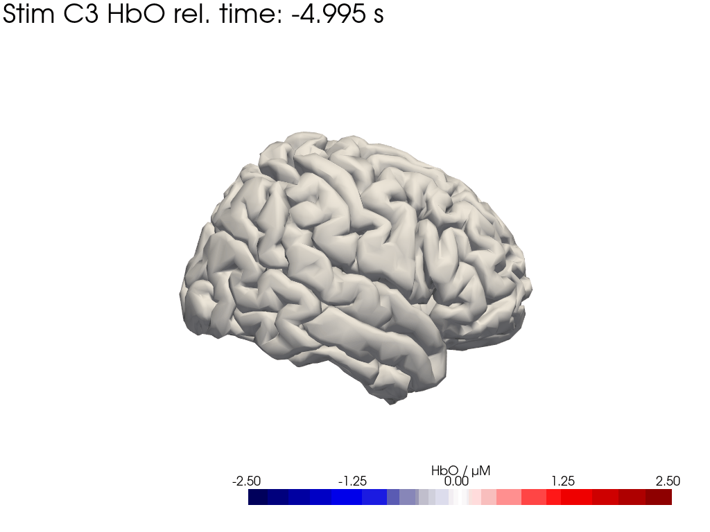
[41]:
display_image("Ftapping-right_HbO_left_hemi.gif")
display_image("Ftapping-right_HbO_right_hemi.gif")
[42]:
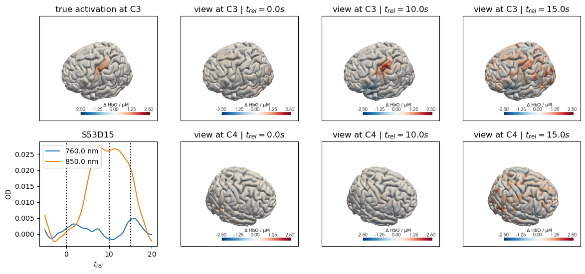
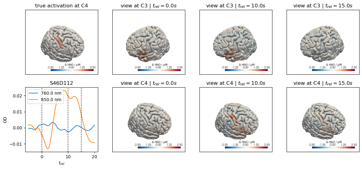
for c, channel in [("C3", roi_chans_c3[-1]), ("C4", roi_chans_c4[-1])]:
    trial_type = f"Stim {c}"

    f,ax = plt.subplots(2,4, figsize=(14,6))
    vmin,vmax = -2.5,2.5

    cedalion.vis.anatomy.plot_brain_in_axes(
        od,
        head_ras.landmarks,
        spatial_imgs.sel(trial_type=trial_type, chromo="HbO").pint.to("uM"),
        head_ras.brain,
        ax[0,0],
        camera_pos=c,
        cmap="RdBu_r",
        vmin=vmin,
        vmax=vmax,
        cb_label=r"$\Delta$ HbO / µM",
        #title=f"{c} Activation",
    )
    ax[0,0].set_title(f"true activation at {c}")

    trels = [0., 10., 15.]
    for i_wl, wl in enumerate(blockaverage.wavelength.values):
        tmp = blockaverage.sel(
            trial_type=trial_type, channel=channel, wavelength=wl
        )
        ax[1,0].plot(tmp.reltime, tmp, label=f"{wl} nm")
    for trel in trels:
        ax[1,0].axvline(trel, c="k", ls=":")
    ax[1,0].legend(loc="upper left")
    ax[1,0].set_xlabel("$t_{rel}$")
    ax[1,0].set_ylabel("OD")
    ax[1,0].set_title(channel)

    for i_col, trel in enumerate(trels, start=1):
        for i_row, cam_pos in enumerate(["C3", "C4"]):
            cedalion.vis.anatomy.plot_brain_in_axes(
                od,
                head_ras.landmarks,
                blockaverage_img.sel(chromo="HbO", trial_type=trial_type)
                .sel(reltime=trel, method="nearest"),
                head_ras.brain,
                ax[i_row, i_col],
                camera_pos=cam_pos,
                cmap="RdBu_r",
                vmin=vmin,
                vmax=vmax,
                cb_label=r"$\Delta$ HbO / µM",
                #title="$t_{rel}=" + f"{trel:.1f} s$",
            )
            ax[i_row, i_col].set_title(f"view at {cam_pos} | " + "$t_{rel}=" + f"{trel:.1f} s$")
Adding Motion Artifacts
The second part of this notebook demonstrates how to add spike and baseline-shift artifacts to existing time series.
First, we’ll load some example data.
[43]:
rec = cedalion.data.get_fingertappingDOT()
rec["od"] = cedalion.nirs.cw.int2od(rec["amp"])

f, ax = plt.subplots(1, 1, figsize=(12, 4))
ax.plot(
    rec["amp"].time,
    rec["amp"].sel(channel="S1D2", wavelength="760"),
    "r-",
    label="760nm",
)
ax.plot(
    rec["amp"].time,
    rec["amp"].sel(channel="S1D2", wavelength="850"),
    "g-",
    label="850nm",
)

plt.legend()
ax.set_xlabel("time / s")
ax.set_ylabel("intensity / V")

display(rec["od"])
<xarray.DataArray (channel: 100, wavelength: 2, time: 8794)> Size: 14MB
[] 0.02263 0.02322 0.01368 0.005969 0.01692 ... 0.01558 0.02343 0.02274 0.02761
Coordinates:
  * time        (time) float64 70kB 0.0 0.2294 0.4588 ... 2.017e+03 2.017e+03
    samples     (time) int64 70kB 0 1 2 3 4 5 ... 8788 8789 8790 8791 8792 8793
  * channel     (channel) object 800B 'S1D1' 'S1D2' 'S1D4' ... 'S14D31' 'S14D32'
    source      (channel) object 800B 'S1' 'S1' 'S1' 'S1' ... 'S14' 'S14' 'S14'
    detector    (channel) object 800B 'D1' 'D2' 'D4' 'D5' ... 'D29' 'D31' 'D32'
  * wavelength  (wavelength) float64 16B 760.0 850.0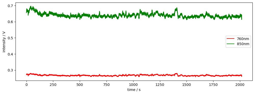
Artifact Generation
Artifacts are generated by the functions gen_bl_shift and gen_spike.
These function take as arguments:
the time axis of time series
onset time
duration
The amplitude of the generated artifacts is set to 1.
[44]:
time = rec["amp"].time
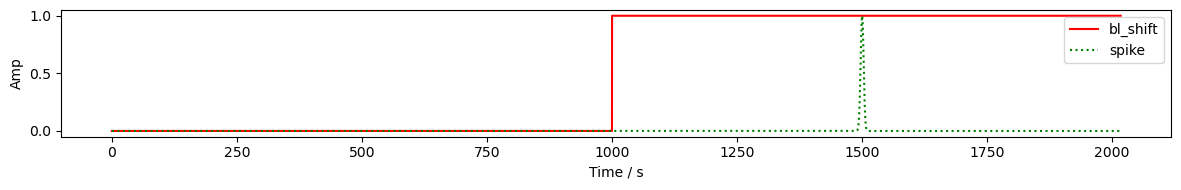
sample_bl_shift = synart.gen_bl_shift(time, 1000) # baseline shift a t = 1000s
sample_spike = synart.gen_spike(time, 1500, 3) # spike artifact at t=1500s for 3s
display(sample_bl_shift)
fig, ax = plt.subplots(1, 1, figsize=(12,2))
ax.plot(time, sample_bl_shift, "r-", label="bl_shift")
ax.plot(time, sample_spike, "g:", label="spike")
ax.set_xlabel('Time / s')
ax.set_ylabel('Amp')
ax.legend()
plt.tight_layout()
plt.show()
<xarray.DataArray 'time' (time: 8794)> Size: 70kB
0.0 0.0 0.0 0.0 0.0 0.0 0.0 0.0 0.0 0.0 ... 1.0 1.0 1.0 1.0 1.0 1.0 1.0 1.0 1.0
Coordinates:
  * time     (time) float64 70kB 0.0 0.2294 0.4588 ... 2.017e+03 2.017e+03
Controlling Artifact Timing
Artifacts can be placed using a timing data frame with columns ‘onset’, ‘duration’, ‘trial_type’, ‘value’, and ‘channel’, i.e. it resembles the stimulus data frame with the added ‘channel’ column.
We can use the function add_event_timing to create such timing data frames. The function allows precise control over each event.
The function sel_chans_by_opt allows us to select a list of channels by way of a list of optode labels. This reflects the fact that motion artifacts usually stem from the motion of a specific optode or set of optodes, which in turn affects all related channels.
We can also use the functions random_events_num and random_events_perc to add random events to the data frame, specifying either the number of events or the percentage of the time series duration, respectively.
[45]:
# Create a list of events in the format (onset, duration)
events = [(1000, 1), (2000, 1)]

# Creates a new timing dataframe with the specified events.
# Setting channel to None indicates that the artifact applies to all channels.
timing_amp = synart.add_event_timing(events, 'bl_shift', None)

# Select channels by optode
chans = synart.sel_chans_by_opt(["S1"], rec["od"])

# Add random events to the timing dataframe
timing_od = synart.random_events_perc(time, 0.01, ["spike"], chans)

display(timing_amp)
display(timing_od)
| onset | duration | trial_type | value | channel | |
|---|---|---|---|---|---|
| 0 | 1000 | 1 | bl_shift | 1 | None |
| 1 | 2000 | 1 | bl_shift | 1 | None |
| onset | duration | trial_type | value | channel | |
|---|---|---|---|---|---|
| 0 | 1915.741510 | 0.244770 | spike | 1 | [S1D1, S1D2, S1D4, S1D5, S1D6, S1D8] |
| 1 | 696.880030 | 0.133781 | spike | 1 | [S1D1, S1D2, S1D4, S1D5, S1D6, S1D8] |
| 2 | 346.574505 | 0.108593 | spike | 1 | [S1D1, S1D2, S1D4, S1D5, S1D6, S1D8] |
| 3 | 1637.416901 | 0.240916 | spike | 1 | [S1D1, S1D2, S1D4, S1D5, S1D6, S1D8] |
| 4 | 1142.925207 | 0.205711 | spike | 1 | [S1D1, S1D2, S1D4, S1D5, S1D6, S1D8] |
| ... | ... | ... | ... | ... | ... |
| 77 | 743.181895 | 0.295253 | spike | 1 | [S1D1, S1D2, S1D4, S1D5, S1D6, S1D8] |
| 78 | 1948.966710 | 0.314755 | spike | 1 | [S1D1, S1D2, S1D4, S1D5, S1D6, S1D8] |
| 79 | 1926.799165 | 0.233208 | spike | 1 | [S1D1, S1D2, S1D4, S1D5, S1D6, S1D8] |
| 80 | 983.910264 | 0.366362 | spike | 1 | [S1D1, S1D2, S1D4, S1D5, S1D6, S1D8] |
| 81 | 297.379197 | 0.265285 | spike | 1 | [S1D1, S1D2, S1D4, S1D5, S1D6, S1D8] |
82 rows × 5 columns
Adding Artifacts to Data
The function add_artifacts scales artifacts and adds them to time-series data.
The artifact generation functions (see above) are passed as a dictionary. Keys correspond to entries in the column ‘trial_type’ of the timing data frame, i.e. each event specified in the timing data frame is generated using the function artifacts[trial_type]. If mode is ‘manual’, artifacts are scaled directly by the scale parameter, otherwise artifacts are automatically scaled by a parameter alpha which is calculated using a sliding window approach.
Finally, artifacts to be added to optical-density time series can be automatically scaled to yield specific concentration amplitudes with the function add_chromo_artifacts_2_od.
[46]:
artifacts = {"spike": synart.gen_spike, "bl_shift": synart.gen_bl_shift}

# Add baseline shifts to the amp data
rec["amp2"] = synart.add_artifacts(rec["amp"], timing_amp, artifacts)

# Convert the amp data to optical density
rec["od2"] = cedalion.nirs.cw.int2od(rec["amp2"])

dpf = xr.DataArray(
    [6, 6],
    dims="wavelength",
    coords={"wavelength": rec["amp"].wavelength},
)

# add spikes to od based on conc amplitudes
rec["od2"] = synart.add_chromo_artifacts_2_od(
    rec["od2"], timing_od, artifacts, rec.geo3d, dpf, 1.5
)

# Plot the OD data
channels = rec["od"].channel.values[0:6]
fig, axes = plt.subplots(len(channels), 1, figsize=(12, len(channels) * 2))
if len(channels) == 1:
    axes = [axes]
for i, channel in enumerate(channels):
    ax = axes[i]
    ax.plot(
        rec["od2"].time,
        rec["od2"].sel(channel=channel, wavelength="850"),
        "g-",
        label="850nm + artifacts",
    )
    ax.plot(
        rec["od"].time,
        rec["od"].sel(channel=channel, wavelength="850"),
        "r-",
        label="850nm - od",
    )
    ax.set_title(f"Channel: {channel}")
    ax.set_xlabel("Time / s")
    ax.set_ylabel("OD")
    ax.legend()
plt.tight_layout()
[47]:
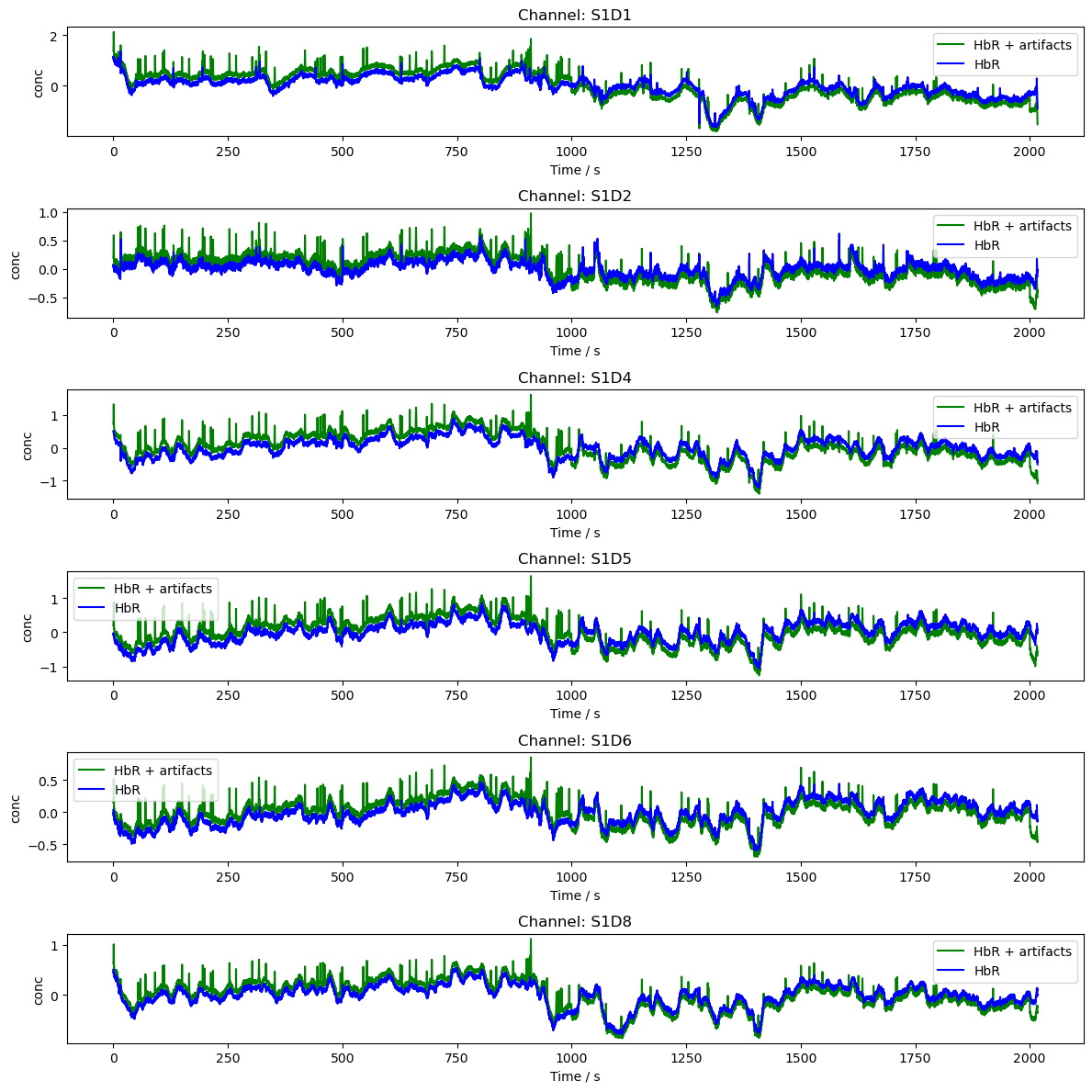
# Plot the data in conc

rec["conc"] = cedalion.nirs.cw.od2conc(rec["od"], rec.geo3d, dpf)
rec["conc2"] = cedalion.nirs.cw.od2conc(rec["od2"], rec.geo3d, dpf)
channels = rec["od"].channel.values[0:6]
fig, axes = plt.subplots(len(channels), 1, figsize=(12, len(channels) * 2))
if len(channels) == 1:
    axes = [axes]
for i, channel in enumerate(channels):
    ax = axes[i]
    ax.plot(
        rec["conc2"].time,
        rec["conc2"].sel(channel=channel, chromo="HbR"),
        "g-",
        label="HbR + artifacts",
    )
    ax.plot(
        rec["conc"].time,
        rec["conc"].sel(channel=channel, chromo="HbR"),
        "b-",
        label="HbR",
    )
    ax.set_title(f"Channel: {channel}")
    ax.set_xlabel("Time / s")
    ax.set_ylabel("conc")
    ax.legend()
plt.tight_layout()
plt.show()
References
[48]:
cedalion.bib.dump_to_notebook()
Methods used
| [1] | Tucker2022 | cedalion.io.snirf.read_snirf | Stephen Tucker, Jay Dubb, Sreekanth Kura, Alexander von Lühmann, Robert Franke, Jörn M. Horschig, Samuel Powell, Robert Oostenveld, Michael Lührs, Édouard Delaire, Zahra M. Aghajan, Hanseok Yun, Meryem A. Yücel, Qianqian Fang, Theodore J. Huppert, Blaise deB. Frederick, Luca Pollonini, David A. Boas, and Robert Luke. Introduction to the shared near infrared spectroscopy format. Neurophotonics, 10(1):013507, 2022. doi:10.1117/1.NPh.10.1.013507. |
| [2] | Huppert2009 | cedalion.sigproc.quality.snr | Theodore J. Huppert, Solomon G. Diamond, Maria A. Franceschini, and David A. Boas. Homer: a review of time-series analysis methods for near-infrared spectroscopy of the brain. Appl. Opt., 48(10):D280–D298, Apr 2009. doi:https://doi.org/10.1364/AO.48.00D280. |
| [3] | Delpy1988 | cedalion.nirs.cw.int2od, cedalion.nirs.cw.od2conc | D. T. Delpy, M. Cope, P. van der Zee, S. Arridge, S. Wray, and J. Wyatt. Estimation of optical pathlength through tissue from direct time of flight measurement. Physics in Medicine and Biology, 33(12):1433–1442, 1988. doi:10.1088/0031-9155/33/12/008. |
| [4] | Villringer1997 | cedalion.nirs.cw.int2od, cedalion.nirs.cw.od2conc | Arno Villringer and Britton Chance. Non-invasive optical spectroscopy and imaging of human brain function. Trends in Neurosciences, 20(10):435–442, 1997. doi:10.1016/S0166-2236(97)01132-6. |
| [5] | Holmes1998 | cedalion.data.get_colin27_headmodel_files | Colin J. Holmes, Rick Hoge, Louis Collins, Roger Woods, Arthur W. Toga, and Alan C. Evans. Enhancement of mr images using registration for signal averaging. Journal of Computer Assisted Tomography, 22(2):324–333, March 1998. doi:10.1097/00004728-199803000-00032. |
| [6] | Fischl2012 | cedalion.data.get_colin27_headmodel_files | Bruce Fischl. FreeSurfer. NeuroImage, 62(2):774–781, 2012. doi:10.1016/j.neuroimage.2012.01.021. |
| [7] | Schaefer2018 | cedalion.data.get_colin27_headmodel_files | Alexander Schaefer, Ru Kong, Evan M Gordon, Timothy O Laumann, Xi-Nian Zuo, Avram J Holmes, Simon B Eickhoff, and BT Thomas Yeo. Local-global parcellation of the human cerebral cortex from intrinsic functional connectivity mri. Cerebral cortex, 28(9):3095–3114, 2018. doi:10.1093/cercor/bhx179. |
| [8] | Gao2015 | cedalion.dataclasses.geometry.PycortexSurface.__init__ | James S. Gao, Alexander G. Huth, Mark D. Lescroart, and Jack L. Gallant. Pycortex: an interactive surface visualizer for fmri. Frontiers in Neuroinformatics, 2015. doi:10.3389/fninf.2015.00023. |
| [9] | Fang2009 | cedalion.data.get_precomputed_sensitivity | Qianqian Fang and David A Boas. Monte carlo simulation of photon migration in 3d turbid media accelerated by graphics processing units. Optics express, 17(22):20178–20190, 2009. doi:10.1364/OE.17.020178. |
| [10] | Yu2018 | cedalion.data.get_precomputed_sensitivity | Leiming Yu, Fanny Nina-Paravecino, David Kaeli, and Qianqian Fang. Scalable and massively parallel monte carlo photon transport simulations for heterogeneous computing platforms. Journal of biomedical optics, 23(1):010504–010504, 2018. doi:10.1117/1.JBO.23.1.010504. |
| [11] | Yan2020 | cedalion.data.get_precomputed_sensitivity | Shijie Yan and Qianqian Fang. Hybrid mesh and voxel based monte carlo algorithm for accurate and efficient photon transport modeling in complex bio-tissues. Biomedical Optics Express, 11(11):6262–6270, 2020. doi:10.1364/BOE.409468. |
| [12] | Prahl1998 | cedalion.nirs.common.get_extinction_coefficients | Scott A. Prahl. Optical absorption of hemoglobin. Oregon Medical Laser Center, online resource, 1998. URL: https://omlc.org/spectra/hemoglobin/. |
| [13] | Strangman2002 | cedalion.models.glm.basis_functions.Gamma.__call__ | Gary Strangman, Joseph P. Culver, John H. Thompson, and David A. Boas. A quantitative comparison of simultaneous BOLD fMRI and NIRS recordings during functional brain activation. NeuroImage, 17(2):719–731, 2002. doi:10.1006/nimg.2002.1227. |
| [14] | Carlton2026 | cedalion.dot.image_recon.ImageRecon.__init__ | Laura B. Carlton, Miray Altınkaynak, Shannon Kelley, Bernhard B. Zimmermann, Sreekanth Kura, Eike Middell, Alexander von Lühmann, Emily P. Stephen, Meryem A. Yücel, and David A. Boas. Surface-based image reconstruction optimization for high-density functional near-infrared spectroscopy. Neurophotonics, 13(2):025001, 2026. doi:10.1117/1.NPh.13.2.025001. |
| [15] | Markow2025 | cedalion.dot.image_recon.ImageRecon.__init__ | Zachary E. Markow, Jason W. Trobaugh, Edward J. Richter, Kalyan Tripathy, Sean M. Rafferty, Alexandra M. Svoboda, Mariel L. Schroeder, Tracy M. Burns-Yocum, Karla M. Bergonzi, Mark A. Chevillet, Emily M. Mugler, Adam T. Eggebrecht, and Joseph P. Culver. Ultra high density imaging arrays in diffuse optical tomography for human brain mapping improve image quality and decoding performance. Scientific Reports, 15(1):3175, January 2025. doi:10.1038/s41598-025-85858-7. |
You have completed the Cedalion tutorial! Return to the tutorial overview or explore the package feature examples.