GLM Basis Functions
[1]:
# This cells setups the environment when executed in Google Colab.
try:
    import google.colab
    !curl -s https://raw.githubusercontent.com/ibs-lab/cedalion/dev/scripts/colab_setup.py -o colab_setup.py
    # Select branch with --branch "branch name" (default is "dev")
    %run colab_setup.py
except ImportError:
    pass
[2]:
import cedalion
import cedalion.models.glm.basis_functions as bf
import cedalion.models.glm.design_matrix as dm

import cedalion.dataclasses as cdc

import matplotlib.pyplot as p
import numpy as np
import xarray as xr
import matplotlib.pyplot as p
import cedalion.data

units = cedalion.units

xr.set_options(display_expand_data=False)
[2]:
<xarray.core.options.set_options at 0x7f75b7392690>
Background: HRF Basis Functions
The General Linear Model (GLM) for fNIRS models the measured haemodynamic time course as a linear combination of regressors. Each regressor is the convolution of a stimulus boxcar function with an HRF basis function — a parametric shape that approximates the expected haemodynamic response to a brief neural event.
Why use multiple basis functions? The haemodynamic response varies across brain regions, subjects, and chromophores. A single fixed shape (e.g. a canonical HRF) may not fit all channels. Using a flexible basis set — several functions spanning a range of latencies and widths — allows the GLM to capture this variability without overfitting.
Cedalion implements the following basis sets in cedalion.models.glm.basis_functions:
Class |
Shape |
Key parameters |
|---|---|---|
|
Set of Gaussian bumps |
|
|
Gaussians + tail components |
as above |
|
Gamma function (physiologically motivated) |
|
|
Gamma + its temporal derivative |
|
|
AFNI-style double-gamma |
|
|
Event-impulse (finite impulse response) |
— |
This notebook visualises each basis set over a trial time window so you can compare their shape and coverage before choosing one for your analysis.
[3]:
# dummy time series
fs = 8.0
ts = cdc.build_timeseries(
    np.random.random((100, 1, 2)),
    dims=["time", "channel", "chromo"],
    time=np.arange(100) / fs,
    channel=["S1D1"],
    value_units=units.uM,
    time_units=units.s,
    other_coords={'chromo' : ["HbO", "HbR"]}
)
display(ts)
<xarray.DataArray (time: 100, channel: 1, chromo: 2)> Size: 2kB
[µM] 0.4779 0.2649 0.5442 0.7449 0.4082 ... 0.3996 0.6961 0.3115 0.6784 0.6714
Coordinates:
  * time     (time) float64 800B 0.0 0.125 0.25 0.375 ... 12.0 12.12 12.25 12.38
    samples  (time) int64 800B 0 1 2 3 4 5 6 7 8 ... 91 92 93 94 95 96 97 98 99
  * channel  (channel) <U4 16B 'S1D1'
* chromo (chromo) <U3 24B 'HbO' 'HbR'[4]:
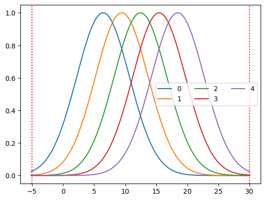
basis = bf.GaussianKernels(
    t_pre=5 * units.s,
    t_post=30 * units.s,
    t_delta=3 * units.s,
    t_std=3 * units.s,
)
hrf = basis(ts)

p.figure()
for i_comp, comp in enumerate(hrf.component.values):
    p.plot(hrf.time, hrf[:, i_comp], label=comp)

p.axvline(-5, c="r", ls=":")
p.axvline(30, c="r", ls=":")
p.legend(ncols=3)
[4]:
<matplotlib.legend.Legend at 0x7f75b4f9df10>

[5]:
basis = bf.GaussianKernelsWithTails(
    t_pre=5 * units.s,
    t_post=30 * units.s,
    t_delta=3 * units.s,
    t_std=3 * units.s,
)
hrf = basis(ts)

p.figure()
for i_comp, comp in enumerate(hrf.component.values):
    p.plot(hrf.time, hrf[:, i_comp], label=comp)
p.axvline(-5, c="r", ls=":")
p.axvline(30, c="r", ls=":")
p.legend(ncols=3)
[5]:
<matplotlib.legend.Legend at 0x7f75b4e6ab50>
[6]:
basis = bf.Gamma(
    tau={"HbO": 0 * units.s, "HbR": 1 * units.s},
    sigma=3 * units.s,
)
hrf = basis(ts)
display(hrf)
p.figure()
for i_comp, comp in enumerate(hrf.component.values):
    for i_chromo, chromo in enumerate(hrf.chromo.values):
        p.plot(hrf.time, hrf[:, i_comp, i_chromo], label=f"{comp} {chromo}")

p.legend()
<xarray.DataArray (time: 107, component: 1, chromo: 2)> Size: 2kB
0.0 0.0 0.004711 0.0 0.01875 ... 2.533e-07 3.574e-06 1.789e-07 2.601e-06
Coordinates:
  * time       (time) float64 856B 0.0 0.125 0.25 0.375 ... 13.0 13.12 13.25
  * chromo     (chromo) <U3 24B 'HbO' 'HbR'
  * component  (component) <U5 20B 'gamma'
[6]:
<matplotlib.legend.Legend at 0x7f75b4edb210>
[7]:
basis = bf.Gamma(
    tau={"HbO": 0 * units.s, "HbR": 1 * units.s},
    sigma=2 * units.s,
)
hrf = basis(ts)
display(hrf)

p.figure()
for i_comp, comp in enumerate(hrf.component.values):
    for i_chromo, chromo in enumerate(hrf.chromo.values):
        p.plot(hrf.time, hrf[:, i_comp, i_chromo], label=f"{comp} {chromo}")

p.legend()
<xarray.DataArray (time: 74, component: 1, chromo: 2)> Size: 1kB
0.0 0.0 0.01058 0.0 0.04181 ... 7.789e-06 8.836e-08 4.894e-06 5.155e-08 3.05e-06
Coordinates:
  * time       (time) float64 592B 0.0 0.125 0.25 0.375 ... 8.75 8.875 9.0 9.125
  * chromo     (chromo) <U3 24B 'HbO' 'HbR'
  * component  (component) <U5 20B 'gamma'
[7]:
<matplotlib.legend.Legend at 0x7f75a9b2b090>
[8]:
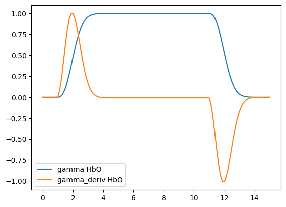
basis = bf.GammaDeriv(
    tau=2 * units.s,
    sigma=2 * units.s,
)
hrf = basis(ts)
display(hrf)
p.figure()
for i_comp, comp in enumerate(hrf.component.values):
    for i_chromo, chromo in enumerate(["HbO"]):
        p.plot(hrf.time, hrf[:, i_comp, i_chromo], label=f"{comp} {chromo}")

p.legend()
<xarray.DataArray (time: 82, component: 2, chromo: 2)> Size: 3kB
0.0 0.0 0.0 0.0 0.0 0.0 ... -2.311e-05 3.05e-06 3.05e-06 -1.466e-05 -1.466e-05
Coordinates:
  * time       (time) float64 656B 0.0 0.125 0.25 0.375 ... 9.875 10.0 10.12
  * chromo     (chromo) <U3 24B 'HbO' 'HbR'
  * component  (component) <U11 88B 'gamma' 'gamma_deriv'
[8]:
<matplotlib.legend.Legend at 0x7f75b505e050>
[9]:
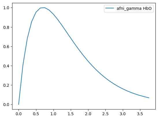
basis = bf.AFNIGamma(
    p=1,
    q=0.7 * units.s,
)
hrf = basis(ts)
display(hrf)
p.figure()
for i_comp, comp in enumerate(hrf.component.values):
    for i_chromo, chromo in enumerate(["HbO"]):
        p.plot(hrf.time, hrf[:, i_comp, i_chromo], label=f"{comp} {chromo}")

p.legend()
<xarray.DataArray (time: 31, component: 1, chromo: 2)> Size: 496B
0.0 0.0 0.407 0.407 0.6809 0.6809 ... 0.0918 0.07953 0.07953 0.06882 0.06882
Coordinates:
  * time       (time) float64 248B 0.0 0.125 0.25 0.375 ... 3.375 3.5 3.625 3.75
  * chromo     (chromo) <U3 24B 'HbO' 'HbR'
  * component  (component) <U10 40B 'afni_gamma'
[9]:
<matplotlib.legend.Legend at 0x7f75a9a0a1d0>

[10]:
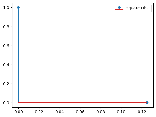
basis = bf.DiracDelta()
hrf = basis(ts)
display(hrf)
p.figure()
for i_comp, comp in enumerate(hrf.component.values):
    for i_chromo, chromo in enumerate(["HbO"]):
        p.stem(hrf.time, hrf[:, i_comp, i_chromo], label=f"{comp} {chromo}")

p.legend()
<xarray.DataArray (time: 2, component: 1, chromo: 2)> Size: 32B
1.0 1.0 0.0 0.0
Coordinates:
  * time       (time) float64 16B 0.0 0.125
  * chromo     (chromo) <U3 24B 'HbO' 'HbR'
  * component  (component) <U6 24B 'square'
[10]:
<matplotlib.legend.Legend at 0x7f75a9a02b50>

References
[11]:
cedalion.bib.dump_to_notebook()
Methods used
| [1] | Strangman2002 | cedalion.models.glm.basis_functions.Gamma.__call__, cedalion.models.glm.basis_functions.GammaDeriv.__call__ | Gary Strangman, Joseph P. Culver, John H. Thompson, and David A. Boas. A quantitative comparison of simultaneous BOLD fMRI and NIRS recordings during functional brain activation. NeuroImage, 17(2):719–731, 2002. doi:10.1006/nimg.2002.1227. |
| [2] | Cox1996 | cedalion.models.glm.basis_functions.AFNIGamma.__call__ | Robert W. Cox. AFNI: software for analysis and visualization of functional magnetic resonance neuroimages. Computers and Biomedical Research, 29(3):162–173, 1996. doi:10.1006/cbmr.1996.0014. |