Scaling and Transforming Head Models

[1]:

# This cells setups the environment when executed in Google Colab.
try:
    import google.colab
    !curl -s https://raw.githubusercontent.com/ibs-lab/cedalion/dev/scripts/colab_setup.py -o colab_setup.py
    # Select branch with --branch "branch name" (default is "dev")
    %run colab_setup.py
except ImportError:
    pass

[2]:

import pyvista as pv

#pv.set_jupyter_backend('server')
pv.set_jupyter_backend('static')

import os

import xarray as xr

import cedalion
import cedalion.data
import cedalion.dataclasses as cdc
import cedalion.dot
import cedalion.io
import cedalion.vis.anatomy
import cedalion.vis.blocks as vbx
from cedalion import units
import numpy as np

xr.set_options(display_expand_data=False);

Loading the ICBM-152 head model

the TwoSurfaceHeadModel holds the segmented MRT image and derived cortex and scalp surfaces
we provide functionality to derive these surfaces from the masks or to load them from files

[3]:

head_ijk = cedalion.dot.get_standard_headmodel("icbm152")
head_ijk

[3]:

TwoSurfaceHeadModel(
  crs: ijk
  tissue_types: csf, gm, scalp, skull, wm
  brain faces: 29978 vertices: 15002 units: dimensionless
  scalp faces: 20040 vertices: 10018 units: dimensionless
  landmarks: 73
)

The head model holds segmentation masks for different tissue types:

[4]:

head_ijk.segmentation_masks

[4]:

<xarray.DataArray (segmentation_type: 5, i: 193, j: 239, k: 263)> Size: 61MB
0 0 0 0 0 0 0 0 0 0 0 0 0 0 0 0 0 0 0 ... 0 0 0 0 0 0 0 0 0 0 0 0 0 0 0 0 0 0 0
Coordinates:
  * segmentation_type  (segmentation_type) <U5 100B 'csf' 'gm' ... 'skull' 'wm'
Dimensions without coordinates: i, j, k

Coordinate System and Transformations

we need to distinguish several coordinate systems: voxel space, scanner space, subject space, …
geometric data types carry information about which crs they use
transformations between coordinate systems through affine transformations

The head model is loaded in voxel space (‘ijk’)

[5]:

head_ijk.crs

[5]:

'ijk'

The head model contains fiducial and 10-10 landmarks stored as LabeledPoints.

The crs is stored as the name of the second dimension, easily retrievable through the .points-accessor

[6]:

display(head_ijk.landmarks)
display(head_ijk.landmarks.points.crs)

<xarray.DataArray (label: 73, ijk: 3)> Size: 2kB
[] 96.0 216.0 105.0 96.0 18.0 118.0 ... 133.1 28.43 182.6 145.1 30.85 166.9
Coordinates:
  * label    (label) <U3 876B 'Nz' 'Iz' 'LPA' 'RPA' ... 'PO1' 'PO2' 'PO4' 'PO6'
    type     (label) object 584B PointType.LANDMARK ... PointType.LANDMARK
Dimensions without coordinates: ijk

'ijk'

Triangulated surface meshes of the scalp and brain:

[7]:

display(head_ijk.brain)
display(head_ijk.scalp)

TrimeshSurface(faces: 29978 vertices: 15002 crs: ijk units: dimensionless vertex_coords: ['parcel'])

TrimeshSurface(faces: 20040 vertices: 10018 crs: ijk units: dimensionless vertex_coords: [])

The affine transformation from voxel to subject (RAS) space:

[8]:

head_ijk.t_ijk2ras

[8]:

<xarray.DataArray (mni: 4, ijk: 4)> Size: 128B
[mm] 1.0 0.0 0.0 -96.0 0.0 1.0 0.0 -132.0 0.0 0.0 1.0 -148.0 0.0 0.0 0.0 1.0
Dimensions without coordinates: mni, ijk

Change to subject (RAS) space by applying an affine transformation on the head model. This transforms all components.

For the ICBM-152 head, the subject space is called ‘mni’. In subject-specific MRI scans the label is derived from information in the masks’ nifti files.

The scanner space also uses physical units whereas coordinates in voxel space are dimensionless.

[9]:

trafo = head_ijk.t_ijk2ras

head_ras = head_ijk.apply_transform(trafo)

display(head_ras)

print(f"Head CRS='{head_ras.crs}'")
print(f"Landmarks CRS='{head_ras.landmarks.points.crs}'")
print(f"Brain surface CRS='{head_ras.brain.crs}'")

print("Landmark units in voxel space:", head_ijk.landmarks.pint.units)
print("Landmark units in scanner space:", head_ras.landmarks.pint.units)

TwoSurfaceHeadModel(
  crs: mni
  tissue_types: csf, gm, scalp, skull, wm
  brain faces: 29978 vertices: 15002 units: millimeter
  scalp faces: 20040 vertices: 10018 units: millimeter
  landmarks: 73
)

Head CRS='mni'
Landmarks CRS='mni'
Brain surface CRS='mni'
Landmark units in voxel space: dimensionless
Landmark units in scanner space: millimeter

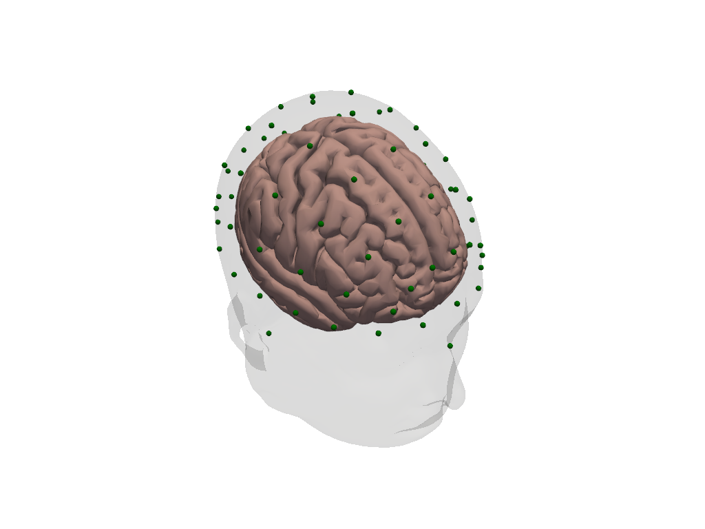
Visualization

[10]:

plt = pv.Plotter()
vbx.plot_surface(plt, head_ijk.brain, color="#d3a6a1")
vbx.plot_surface(plt, head_ijk.scalp, opacity=.1)
vbx.plot_labeled_points(plt, head_ijk.landmarks, show_labels=True)
plt.show()

../../_images/examples_head_models_43_crs_and_headmodel_18_0.png

Scaling head models and optode positions

[11]:

def compare_trafos(t_orig, t_scaled):
    """Compare the length of a unit vector after applying the transform."""
    t_orig = t_orig.pint.dequantify().values
    t_scaled = t_scaled.pint.dequantify().values

    for i, dim in enumerate("xyz"):
        unit_vector = np.zeros(4)
        unit_vector[i] = 1.0
        n1 = np.linalg.norm(t_orig @ unit_vector)
        n2 = np.linalg.norm(t_scaled @ unit_vector)

        print(
            f"After scaling a unit vector along the {dim}-axis is {n2 / n1 * 100.0:.1f}% "
            "of the original length."
        )

Scale head model using geodesic distances

Transform the head model to the subject’s head size as defined by three measurements:

the head circumference
the distance from Nz through Cz to Iz
the distance from LPA through Cz to RPA

These distances define a ellipsoidal scalp surface to which the head model is fit.

The resulting head will be in CRS=’ellipsoid’.

[12]:

head_scaled = head_ijk.scale_to_headsize(
    circumference=51*units.cm,
    nz_cz_iz=33*units.cm,
    lpa_cz_rpa=33*units.cm
)

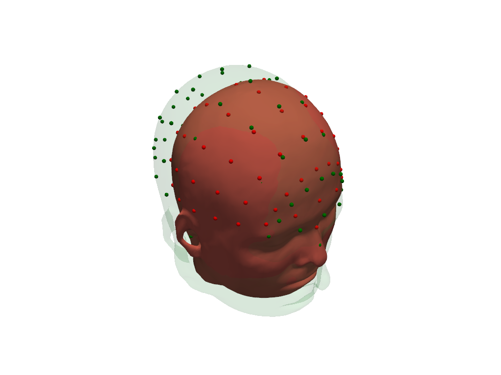
Visualize original (green) and scaled (red) scalp surfaces and landmarks.

[13]:

plt = pv.Plotter()
vbx.plot_surface(plt, head_ras.scalp, color="#4fce64", opacity=.1)
vbx.plot_labeled_points(plt, head_ras.landmarks, color="g")
vbx.plot_surface(plt, head_scaled.scalp, color="#ce5c4f")
vbx.plot_labeled_points(plt, head_scaled.landmarks, color="r")
plt.show()

../../_images/examples_head_models_43_crs_and_headmodel_25_0.png

[14]:

compare_trafos(head_ijk.t_ijk2ras, head_scaled.t_ijk2ras)

After scaling a unit vector along the x-axis is 102.2% of the original length.
After scaling a unit vector along the y-axis is 77.9% of the original length.
After scaling a unit vector along the z-axis is 85.1% of the original length.

Scale head model using digitized landmark positions

Transform the head model to the subject’s head size by fitting landmarks of the head model to digitized landmarks.

The resulting head will be in the same CRS as the digitized landmarks. This also affects axis orientations.

[15]:

# Construct LabeledPoints with landmark positions.
# Use the digitized landmarks from 41_photogrammetric_optode_coregistration.ipynb
geo3d = cdc.build_labeled_points(
    [
        [14.00420712, -7.84856869, 449.77840004],
        [99.09920059, 29.72154755, 620.73876117],
        [161.63815139, -48.49738938, 494.91210993],
        [82.8771277, 79.79500128, 498.3338802],
        [15.17214095, -60.56186128, 563.29621021],
    ],
    crs="digitized",
    labels=["Nz", "Iz", "Cz", "LPA", "RPA"],
    types = [cdc.PointType.LANDMARK] * 5,
    units="mm"
)

# shift the center of the landmarks to plot original and
# scaled versions next to each other
geo3d = geo3d - geo3d.mean("label") + (0,200,0)*cedalion.units.mm

head_scaled = head_ijk.scale_to_landmarks(geo3d)

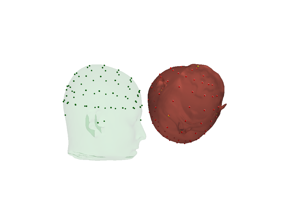
Visualize original (green) and scaled (red) scalp surfaces and landmarks.

The digitized landmarks are plotted in yellow.

[16]:

plt = pv.Plotter()
vbx.plot_surface(plt, head_ras.scalp, color="#4fce64", opacity=.1)
vbx.plot_labeled_points(plt, head_ras.landmarks, color="g")
vbx.plot_surface(plt, head_scaled.scalp, color="#ce5c4f", opacity=.8)
vbx.plot_labeled_points(plt, head_scaled.landmarks, color="r")
vbx.plot_labeled_points(plt, geo3d, color="y", )
vbx.camera_at_cog(plt, head_scaled.scalp, (600,0,0), fit_scene=True)
plt.show()

../../_images/examples_head_models_43_crs_and_headmodel_30_0.png

[17]:

compare_trafos(head_ijk.t_ijk2ras, head_scaled.t_ijk2ras)

After scaling a unit vector along the x-axis is 111.8% of the original length.
After scaling a unit vector along the y-axis is 97.8% of the original length.
After scaling a unit vector along the z-axis is 90.2% of the original length.

Scale digitized optode positions to head model

Load a fingertapping dataset to obtain digitized optode coordinates in a different coordinate system.

[18]:

rec = cedalion.data.get_fingertappingDOT()

display(rec.geo3d)
print(f"The optodes' coordinate refernce system is CRS='{rec.geo3d.points.crs}'.")

<xarray.DataArray (label: 346, digitized: 3)> Size: 8kB
[mm] -77.82 15.68 23.17 -61.91 21.23 56.49 ... 14.23 -38.28 81.95 -0.678 -37.03
Coordinates:
    type     (label) object 3kB PointType.SOURCE ... PointType.LANDMARK
  * label    (label) <U6 8kB 'S1' 'S2' 'S3' 'S4' ... 'FFT10h' 'FT10h' 'FTT10h'
Dimensions without coordinates: digitized

The optodes' coordinate refernce system is CRS='digitized'.

Without changing the head model size, transform the optode positions to fit the head model’s landmarks.

This function calculates an unconstrained affine transformation to bring landmarks as best as possible into alignment. Any remaining distance between transformed optode positions from the scalp surface is removed by snapping each transformed optode to its nearest scalp vertex.

To derive the unconstrained transformation the digitized coordinates and head model landmarks must contain at least the positions of “Nz”, “Iz”, “Cz”, “LPA”, “RPA”.

If less landmarks are available align_and_snap_to_scalp can be called with mode='trans_rot_isoscale, which restricts the affine to translations, rotations and isotropic scaling, which have less degrees of freedom.

[19]:

geo3d_snapped = head_ras.align_and_snap_to_scalp(rec.geo3d)

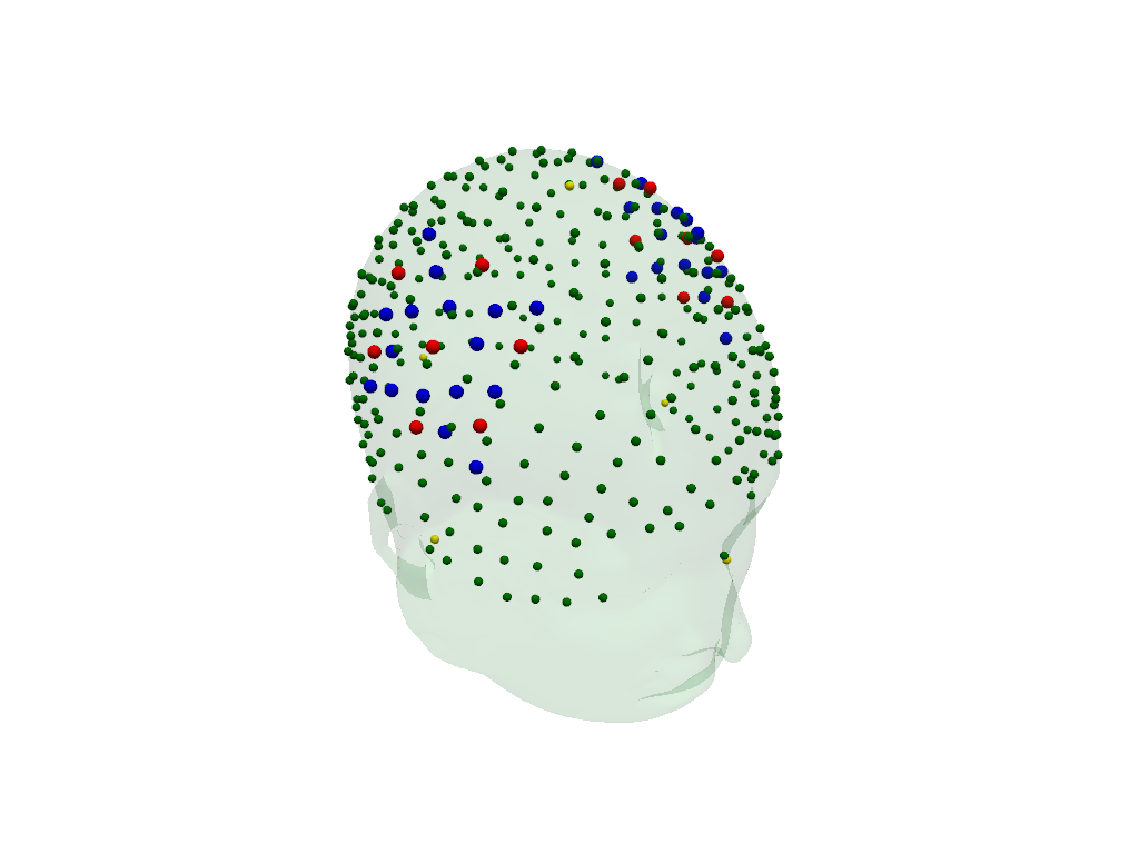
The transformed digitized optode and landmark positions are plotted in red (sources), blue (detectors) and green (landmarks).

The fiducial landmarks of the head model are plotted in yellow.

[20]:

plt = pv.Plotter()
vbx.plot_surface(plt, head_ras.scalp, color="#4fce64", opacity=.1)
vbx.plot_labeled_points(plt, geo3d_snapped)
vbx.plot_labeled_points(
    plt, head_ras.landmarks.sel(label=["Nz", "Iz", "Cz", "LPA", "RPA"]), color="y"
)
plt.show()

../../_images/examples_head_models_43_crs_and_headmodel_38_0.png

Magnitude	[[1.0 0.0 0.0 -96.0] [0.0 1.0 0.0 -132.0] [0.0 0.0 1.0 -148.0] [0.0 0.0 0.0 1.0]]
Units	millimeter

Magnitude	[[-77.817871 15.680613999999998 23.172269999999997] [-61.906841 21.227732000000003 56.492802] [-85.37146 -16.079958 8.900885] ... [77.521 28.883 -39.113] [80.59 14.229 -38.278] [81.95 -0.678 -37.027]]
Units	millimeter