MRI T1 Processing and Segmentation Documentation
This documentation explains the workflow for MRI image segmentation for subsequent use within Cedalion.
The Cedalion head model workflows, as exemplarily described by the jupyter notebooks 40_image_reconstruction.ipynb, 41_photogrammetric_optode_coregistration.ipynb, 42_1010_system.ipynb, 43_crs_and_headmodel.ipynb, 44_head_models.ipynb, 45_parcel_sensitivity.ipynb, 46_precompute_fluence.ipynb, require either standard or individual head models, built from raw MRI images through a series of segmentation, post-processing, meshing, cortical surface extraction and parcellation labeling steps.
Overview of the Processing Workflows
The workflows integrate multiple tools outside Python, including Brainstorm, CAT12, and FreeSurfer, for sequential processing of MRI data. This documentation provides a step-by-step guide to help ensure efficient data preparation, segmentation, and model alignment.
Workflow 1: Nils full Workflow in MATLAB
Nils has a repository (harmening/MRIsegmentation) which contains a fully automatic MATLAB workflow for MRI segmentation (using SPM and CAT12), postprocessing, mesh generation and brain parcellation labeling. The README contains all information about how to install and start the
segmentation (running start_segmentation_cedalion(<<path-to-MRI.nii>>) is sufficient). Output: Post-processed 6-type tissue segmentation masks (mask_air.nii, mask_skin.nii, mask_bone.nii, mask_csf.nii, mask_gray.nii, mask_white.nii), scalp and brain surfaces (mask_scalp.obj, mask_scalp.obj) and Schaefer2018 parcellation labels (parcels.json), that
can be directly loaded into cedalion.
Workflow 2: CAT12 in Brainstorm + Freesurfer
Step 1: T1 Image Segmentation
MRI segmentation is the process of partitioning an MRI scan into the different biological tissue types. The neuroscience community so far developed various powerful tools to segment a T1-weighted MRI image that all exhibit different strengths and weaknesses. We present two of them here shortly additional to Nils workflow, where each of them is suffient. However, we usually do the segmentation with using both Nils workflow and CAT12 in Brainstorm and choose the best one. For a detailed brain surface model we sometimes additionally add the FreeSurfer workflow.
A: CAT12 in Brainstorm
Brainstorm Overview: Brainstorm is an open-source application designed for the analysis of brain recordings. It can be used as a standalone version or installed via MATLAB, and is integral to many neuroimaging workflows. It makes it easy to perform SPM, CAT12 and Freesurfer analysis.
- CAT12 Toolbox:CAT12 is a computational toolbox that extends the SPM (Statistical Parametric Mapping) software package and is primarily used for structural MRI (sMRI) analysis. CAT12 automates many preprocessing steps required for sMRI, including:
Tissue segmentation into six types (skull, scalp, cerebrospinal fluid (CSF), gray matter, white matter, and air).
Normalization and modulation of images.
Surface generation for brain and head models.
Output from CAT12 used in cedalion: CAT12’s outputted 6-type tissue segmentations (skull, scalp, CSF, gray matter, white matter, and air) and the generated head surface.
B: Detailed Analysis with FreeSurfer
- FreeSurfer Overview:FreeSurfer is a widely-used software package in neuroimaging, specifically for MRI structural analysis. Known for its precise and reproducible methods, FreeSurfer is used to segment brain structures, reconstruct cortical surfaces, and quantify cortical thickness, surface area, and volume.
- Run Segmentation:Download and install FreeSurfer. To do the segmentation run
# Define your FREESURFER_HOME environment variable (if you havn't done already during installation)
export FREESURFER_HOME=/path/to/FreeSurfer
source $FREESURFER_HOME/SetUpFreeSurfer.sh

# Tell FreeSurfer where to put the segmentation results
export SUBJECTS_DIR=/path/to/your/subjects_dir

# Start segmentation
my_subject=sample
my_NIfTI=/path/to/NIfTI.nii.gz
recon-all -i $my_NIfTI -s $my_subject -all
Processing Outputs: In this workflow, FreeSurfer provides details including:
Cortical and subcortical segmentation
Gray and white matter segmentation
Detailed brain surface model
Key Outputs from FreeSurfer: Cedalion’s workflow uses FreeSurfer’s gray matter and white matter segmentations and its detailed brain surface model.
Step 2: Parcellation using Schaefer Atlas
The Schaefer Atlas is a popular parcellation scheme for the human brain used in neuroimaging research. It was developed by Schaefer et al. (2018) and provides a fine-grained parcellation of the cortex based on functional connectivity data from resting-state fMRI. One of the distinctive features of the Schaefer Atlas is its organization of brain regions into well-defined networks that reflect patterns of correlated brain activity. The atlas offers two primary options for network parcellation:
Schaefer Atlas with 7 Networks This version divides the brain into 7 broad functional networks. Often used in studies where the focus is on high-level brain networks, such as understanding large-scale brain organization, general connectivity patterns, or when simplifying data for group analyses.
Schaefer Atlas with 17 Networks This version provides a more granular division of the brain into 17 functional networks. These include the original 7 networks, but with further subdivisions. Suitable for studies that require more detailed parcellation to capture subtle differences in brain function, such as exploring intra-network connectivity or specific functional regions within the brain’s broader networks.
Parcellations are computed in Freesurfer.
Step 3: Alignment and Optimization in Brainstorm
- Data Alignment:To ensure consistency, outputs from CAT12 and FreeSurfer are loaded into Brainstorm, where tissue segmentation files and surfaces are aligned to MNI coordinates. This step is crucial for integrating data accurately within Cedalion’s models.
- Mesh Optimization:Since FreeSurfer surfaces contain ~300K vertices, we downsample the mesh in Brainstorm to a more manageable 15K vertices, which balances detail and processing efficiency in Cedalion.
Step 4: Post-Processing of Tissue Segmentation Masks
- Post-Processing Workflow:To finalize tissue segmentation masks, Cedalion applies additional post-processing steps to smoothen boundaries and fill small gaps. These operations ensure cleaner and more continuous tissue delineation.
Preservation of Key Segmentations:
Gray and White Matter: FreeSurfer’s gray and white matter segmentations are retained without modification due to their high accuracy. Final checks are applied to prevent overlap between masks and to ensure clarity in tissue delineation.
Final Outputs
For each T1 image, the workflow yields the following:
6 Tissue Segmentation Masks: skull, scalp, CSF, gray matter, white matter, and air (air mask optional).
Head Surface and Brain Surface
Parcellations json file
Note that the brain surface, along with gray and white matter masks, originates from FreeSurfer. All other segmentation masks and the head surface are generated from CAT12.
The flowchart below provides a visual summary of this processing pipeline.

[1]:
# This cells setups the environment when executed in Google Colab.
try:
    import google.colab
    !curl -s https://raw.githubusercontent.com/ibs-lab/cedalion/dev/scripts/colab_setup.py -o colab_setup.py
    # Select branch with --branch "branch name" (default is "dev")
    %run colab_setup.py
except ImportError:
    pass
[2]:
# load dependencies

import pyvista as pv
import os

import cedalion
import cedalion.io
import cedalion.vis.blocks as vbx
import cedalion.data
from cedalion.dot import TwoSurfaceHeadModel
import cedalion.dataclasses as cdc


import numpy as np

import nibabel as nib
from nilearn import plotting as niplotting

# pv.set_jupyter_backend('client')
pv.set_jupyter_backend('static')
Colin 27
The Colin27 head is a high-resolution, standardized anatomical brain template based on a series of MRI scans from a single individual, known as “Colin.” The final dataset was created by averaging 27 separate scans of Colin’s brain, resulting in an exceptionally high signal-to-noise ratio and high anatomical detail.
Limitations of the Colin27 Head
Single-Subject Template: Because Colin27 is based on a single individual, it may not represent anatomical variations found in a broader population. Templates like MNI152 or the ICBM (International Consortium for Brain Mapping) average, which are based on multiple subjects, may be preferred in population studies.
Older MRI Technology: The Colin27 scans were acquired in the 1990s using MRI technology of that time, which, while high-quality, may not match the resolution possible with modern imaging techniques.
Plotting
Creating Two-Surface Head Model
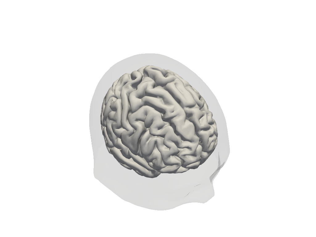
Using from_surfaces method
This method utilizes the brain surface extracted from Freesurfer analysis and the head surface extracted from CAT12. Note that if either of the surface files are not provided it uses the segmentation files.
[3]:
# load segmentation data from the colin27 atlas
SEG_DATADIR_cl27, mask_files_cl27, landmarks_file_cl27 = cedalion.data.get_colin27_segmentation()
PARCEL_DIR_cl27 = cedalion.data.get_colin27_parcel_file()
[4]:
SEG_DATADIR_cl27
[4]:
'/home/eike/.cache/cedalion/dev/colin27_segmentation.zip.unzip/colin27_segmentation'
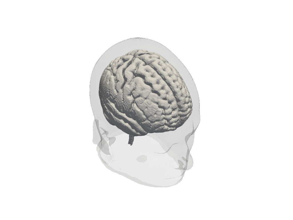
Using from_segmentations method
This method utilizes tissue segmentation files and creates brain and head surfaces from the provided masks.
[5]:
head_colin27 = TwoSurfaceHeadModel.from_segmentation(
    segmentation_dir=SEG_DATADIR_cl27,
    mask_files = mask_files_cl27,
    landmarks_ras_file=landmarks_file_cl27,
    brain_face_count=None,
    scalp_face_count=None,
)
[6]:
head_colin27.brain.vertices
[6]:
<xarray.DataArray (label: 316922, ijk: 3)> Size: 8MB
<Quantity([[ 15.89999962  84.          62.        ]
 [ 16.          84.          61.90000153]
 [ 16.          83.90000153  62.        ]
 ...
 [162.1000061  108.          59.        ]
 [162.1000061  108.          60.        ]
 [163.1000061  105.          61.        ]], 'dimensionless')>
Coordinates:
  * label    (label) int64 3MB 0 1 2 3 4 ... 316917 316918 316919 316920 316921
Dimensions without coordinates: ijk
[7]:
# plot Colin headmodel
plt = pv.Plotter()
vbx.plot_surface(plt, head_colin27.brain, color="w")
vbx.plot_surface(plt, head_colin27.scalp, opacity=.1)
plt.show()

[8]:
# create forward model class for colin 27 atlas
head_colin27 = TwoSurfaceHeadModel.from_surfaces(
    segmentation_dir=SEG_DATADIR_cl27,
    mask_files = mask_files_cl27,
    brain_surface_file= os.path.join(SEG_DATADIR_cl27, "mask_brain.obj"),
    scalp_surface_file= os.path.join(SEG_DATADIR_cl27, "mask_scalp.obj"),
    landmarks_ras_file=landmarks_file_cl27,
    brain_face_count=None,
    scalp_face_count=None,
    parcel_file=PARCEL_DIR_cl27
)
[9]:
# plot Colin headmodel
plt = pv.Plotter()
vbx.plot_surface(plt, head_colin27.brain, color="w")
vbx.plot_surface(plt, head_colin27.scalp, opacity=.1)
plt.show()
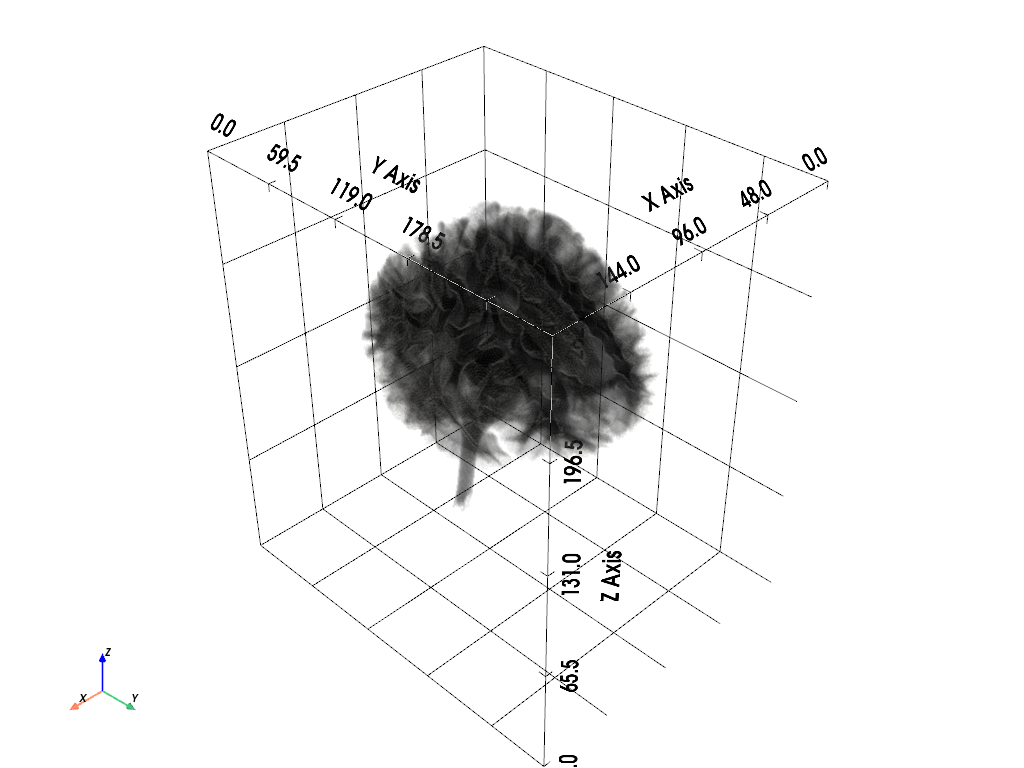
We can also visualize different tisue segmentation volumes.
[10]:
colin27_mask_data = (
    head_colin27.segmentation_masks.sel(segmentation_type="wm")
    + head_colin27.segmentation_masks.sel(segmentation_type="gm")
    + head_colin27.segmentation_masks.sel(segmentation_type="csf")
    + head_colin27.segmentation_masks.sel(segmentation_type="scalp")
    + head_colin27.segmentation_masks.sel(segmentation_type="skull")
)

mask_data = colin27_mask_data.values

# Create a PyVista ImageData object with correct dimensions
grid = pv.ImageData(dimensions=mask_data.shape)
grid.spacing = (1.0, 1.0, 1.0)  # Replace with actual voxel dimensions if available

flattened_mask_data = mask_data.flatten(order="F")

# Choose the specific label to visualize (e.g., Label 2 for 'gm')
label_to_visualize = 5
binary_mask = np.where(flattened_mask_data == label_to_visualize, 1.0, 0.0)

# Add binary mask to the grid as 'SpecificLabel'
grid.point_data["SpecificLabel"] = binary_mask.astype(float) * 100

# Plotting
plotter = pv.Plotter()
# Adding the volume with the appropriate opacity mapping

plotter.add_volume(
    grid,
    scalars="SpecificLabel",
    cmap="Greys",
    clim=[0, 255],
    opacity=[0.0, 0.3],
    shade=True,
    show_scalar_bar=False,
)

plotter.add_axes()
plotter.show_bounds(grid=True)
plotter.show()

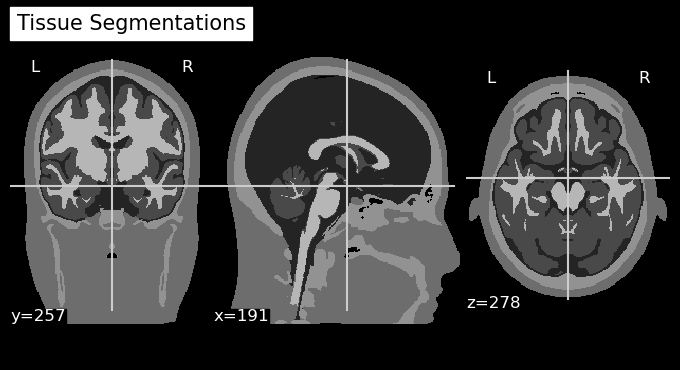
[11]:
mri_img = nib.Nifti1Image(colin27_mask_data, affine=head_colin27.t_ras2ijk)

# Plot the Anatomy
niplotting.plot_anat(mri_img, display_mode='ortho', title='Tissue Segmentations')
niplotting.show()
/opt/miniconda3/envs/cedalion_250922/lib/python3.11/site-packages/xarray/core/variable.py:315: UnitStrippedWarning: The unit of the quantity is stripped when downcasting to ndarray.
  data = np.asarray(data)

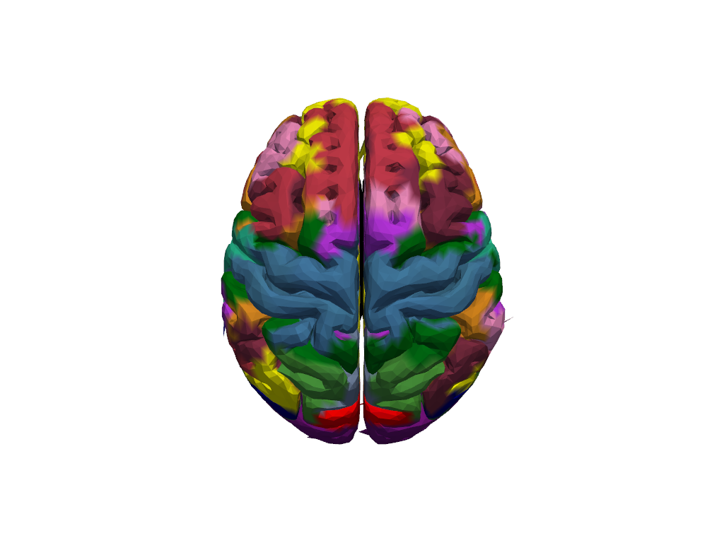
Plot Parcellations
Plot the whole brain surface with their projected parcellations and related colors provided bu Schaefer Atlas. There are almost 600 different colors in this plot but the neighbor regions have near color codes; therefore, it might be difficult to distinguish the borders.
[12]:
parcels = cedalion.io.read_parcellations(PARCEL_DIR_cl27)
[13]:
b = cdc.VTKSurface.from_trimeshsurface(head_colin27.brain)
b = pv.wrap(b.mesh)
b["parcels"] = parcels.Color.tolist()

plt = pv.Plotter()

plt.add_mesh(
    b,
    scalars="parcels",
    rgb=True,
    silhouette=True,
    smooth_shading=True,
)

cog = head_colin27.brain.vertices.mean("label").values

plt.camera.position = cog + [0, 0, 400]
plt.camera.focal_point = cog
plt.camera.up = [0, 1, 0]
plt.reset_camera()

plt.show()
/opt/miniconda3/envs/cedalion_250922/lib/python3.11/site-packages/xarray/core/variable.py:315: UnitStrippedWarning: The unit of the quantity is stripped when downcasting to ndarray.
  data = np.asarray(data)

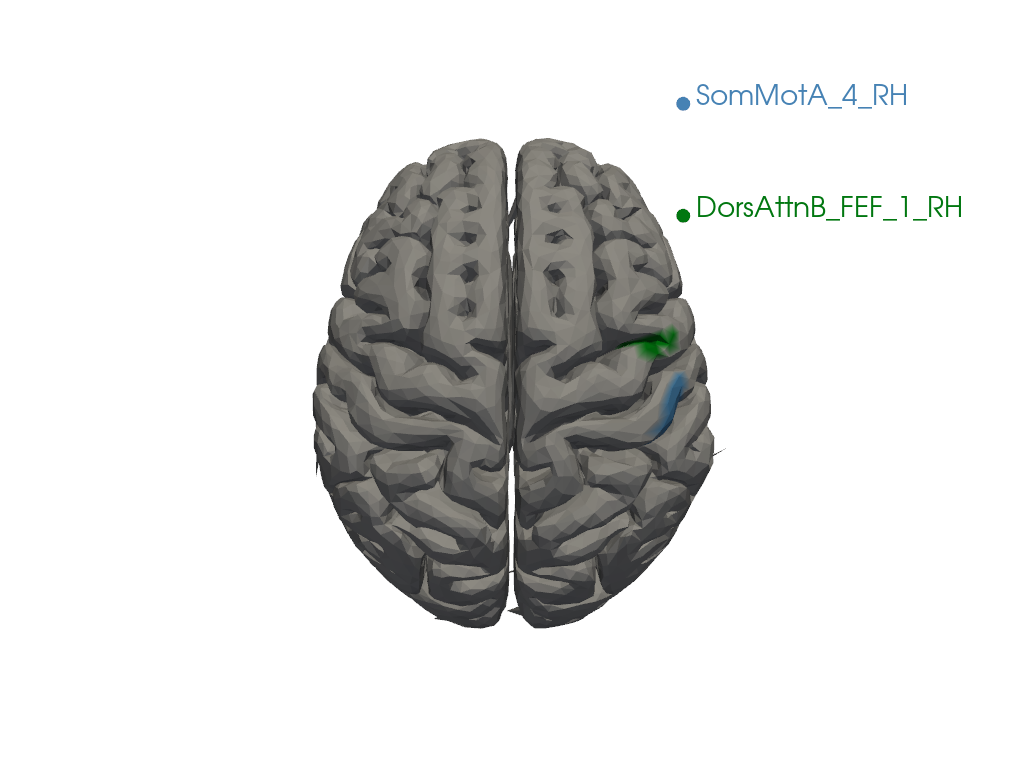
Plot the brain surface with a list of desired parcellations
To better understand the borders, you can specify a list of parcellation names. In the code section below, two regions ("17Networks_RH_SomMotA_4", "17Networks_RH_DorsAttnB_FEF_1") have been selected as examples. You can modify these names or add more regions as needed.
[14]:
parcel_labels = parcels[["Color", "Label"]].drop_duplicates("Label").set_index("Label")
selected_parcels = ["SomMotA_5_RH", "SomMotA_5_LH"]
parcel_colors = parcel_labels.loc[selected_parcels].to_dict("dict")['Color']

b = cdc.VTKSurface.from_trimeshsurface(head_colin27.brain)
b = pv.wrap(b.mesh)
b["parcels"] = np.asarray([
    parcel_colors.get(parcel, (0.8, 0.8, 0.8))
    for parcel in head_colin27.brain.vertices.parcel.values
])

plt = pv.Plotter()

plt.add_mesh(b, scalars="parcels", rgb=True, smooth_shading=True, silhouette=True)

legends = tuple([list(a) for a in zip(parcel_colors.keys(),parcel_colors.values())])
plt.add_legend(labels=legends, face="o", size=(0.3, 0.3))

cog = head_colin27.brain.vertices.mean("label").values

plt.camera.position = cog + [0,0,400]
plt.camera.focal_point = cog
plt.camera.up = [0,1,0]
plt.reset_camera()

plt.show()
/opt/miniconda3/envs/cedalion_250922/lib/python3.11/site-packages/xarray/core/variable.py:315: UnitStrippedWarning: The unit of the quantity is stripped when downcasting to ndarray.
  data = np.asarray(data)

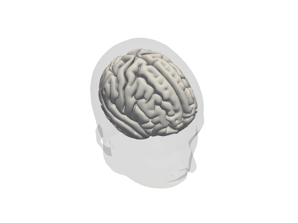
ICBM 152
ICBM152 is a template widely used as a standard brain reference in neuroimaging. Unlike the older Colin27, which is based on a single individual’s MRI scans, the ICBM152 template is created from the averaged MRI scans of 152 healthy adult brains, which makes it more representative of the general population.
Limitations
Still Population-Based: While ICBM152 2020 is more generalizable than single-subject templates, it still represents an average of a specific sample, which may not perfectly match individual brains, particularly those outside the demographic profile used for the template.
Not Always Suitable for Pediatric or Clinical Populations: ICBM152 2020 is based on adult brains, so studies involving pediatric, elderly, or clinical populations with specific pathologies may require alternative templates for more accurate representation.
[15]:
# load segmentation data from the icbm152 atlas
SEG_DATADIR_ic152, mask_files_ic152, landmarks_file_ic152 = cedalion.data.get_icbm152_segmentation()
PARCEL_DIR_ic152 = cedalion.data.get_icbm152_parcel_file()
[16]:
# create forward model class for icbm152 atlas
head_icbm152 = TwoSurfaceHeadModel.from_segmentation(
    segmentation_dir=SEG_DATADIR_ic152,
    mask_files=mask_files_ic152,
    landmarks_ras_file=landmarks_file_ic152,
    brain_face_count=None,
    scalp_face_count=None,
)
[17]:
# plot ICBM headmodel
plt = pv.Plotter()
vbx.plot_surface(plt, head_icbm152.brain, color="w")
vbx.plot_surface(plt, head_icbm152.scalp, opacity=.1)
plt.show()
[18]:
# create forward model class for icbm152 atlas
head_icbm152 = TwoSurfaceHeadModel.from_surfaces(
    segmentation_dir=SEG_DATADIR_ic152,
    mask_files=mask_files_ic152,
    brain_surface_file=os.path.join(SEG_DATADIR_ic152, "mask_brain.obj"),
    scalp_surface_file=os.path.join(SEG_DATADIR_ic152, "mask_scalp.obj"),
    landmarks_ras_file=landmarks_file_ic152,
    brain_face_count=None,
    scalp_face_count=None,
    parcel_file=PARCEL_DIR_ic152,
    smoothing=0,
)
[19]:
# plot ICBM headmodel
plt = pv.Plotter()
vbx.plot_surface(plt, head_icbm152.brain, color="w")
vbx.plot_surface(plt, head_icbm152.scalp, opacity=.1)
plt.show()
[20]:
icbm152_mask_data = (
    head_icbm152.segmentation_masks.sel(segmentation_type="wm")
    + head_icbm152.segmentation_masks.sel(segmentation_type="gm")
    + head_icbm152.segmentation_masks.sel(segmentation_type="csf")
    + head_icbm152.segmentation_masks.sel(segmentation_type="scalp")
    + head_icbm152.segmentation_masks.sel(segmentation_type="skull")
)

mask_data = icbm152_mask_data.values

# Create a PyVista ImageData object with correct dimensions
grid = pv.ImageData(dimensions=mask_data.shape)
grid.spacing = (1.0, 1.0, 1.0)  # Replace with actual voxel dimensions if available

flattened_mask_data = mask_data.flatten(order="F")

# Choose the specific label to visualize (e.g., Label 2 for 'gm')
label_to_visualize = 5
binary_mask = np.where(flattened_mask_data == label_to_visualize, 1.0, 0.0)

# Add binary mask to the grid as 'SpecificLabel'
grid.point_data["SpecificLabel"] = binary_mask.astype(float) * 100

# Plotting
plotter = pv.Plotter()
# Adding the volume with the appropriate opacity mapping

plotter.add_volume(
    grid,
    scalars="SpecificLabel",
    cmap="Greys",
    clim=[0, 255],
    opacity=[0.0, 0.3],
    shade=True,
    show_scalar_bar=False,
)

plotter.add_axes()
plotter.show_bounds(grid=True)
plotter.show()
[21]:
mri_img = nib.Nifti1Image(icbm152_mask_data, affine=head_icbm152.t_ras2ijk)

# Plot the Anatomy
niplotting.plot_anat(mri_img, display_mode='ortho', title='Tissue Segmentations')
niplotting.show()
/opt/miniconda3/envs/cedalion_250922/lib/python3.11/site-packages/xarray/core/variable.py:315: UnitStrippedWarning: The unit of the quantity is stripped when downcasting to ndarray.
  data = np.asarray(data)
[22]:
parcels = cedalion.io.read_parcellations(PARCEL_DIR_ic152)
[23]:
b = cdc.VTKSurface.from_trimeshsurface(head_icbm152.brain)
b = pv.wrap(b.mesh)
b["parcels"] = parcels.Color.tolist()

plt = pv.Plotter()

plt.add_mesh(b, scalars="parcels", rgb=True, smooth_shading=True, silhouette=True)

cog = head_icbm152.brain.vertices.mean("label").values

plt.camera.position = cog + [0, 0, 400]
plt.camera.focal_point = cog
plt.camera.up = [0, 1, 0]
plt.reset_camera()

plt.show()
/opt/miniconda3/envs/cedalion_250922/lib/python3.11/site-packages/xarray/core/variable.py:315: UnitStrippedWarning: The unit of the quantity is stripped when downcasting to ndarray.
  data = np.asarray(data)
[24]:
parcel_labels = parcels[["Color", "Label"]].drop_duplicates("Label").set_index("Label")
selected_parcels = ["SomMotA_5_RH", "SomMotA_5_LH"]
parcel_colors = parcel_labels.loc[selected_parcels].to_dict("dict")['Color']

b = cdc.VTKSurface.from_trimeshsurface(head_icbm152.brain)
b = pv.wrap(b.mesh)
b["parcels"] = np.asarray([
    parcel_colors.get(parcel, (0.8, 0.8, 0.8))
    for parcel in head_icbm152.brain.vertices.parcel.values
])

plt = pv.Plotter()

plt.add_mesh(b, scalars="parcels", rgb=True, smooth_shading=True, silhouette=True)

legends = tuple([list(a) for a in zip(parcel_colors.keys(),parcel_colors.values())])
plt.add_legend(labels=legends, face="o", size=(0.3, 0.3))

cog = head_icbm152.brain.vertices.mean("label").values

plt.camera.position = cog + [0, 0, 400]
plt.camera.focal_point = cog
plt.camera.up = [0, 1, 0]
plt.reset_camera()

plt.show()
/opt/miniconda3/envs/cedalion_250922/lib/python3.11/site-packages/xarray/core/variable.py:315: UnitStrippedWarning: The unit of the quantity is stripped when downcasting to ndarray.
  data = np.asarray(data)