AMPD - Automatic Multiscale Peak Detection
This notebook provides an end-to-end pipeline for processing and analyzing fNIRS data collected during a finger-tapping task. The primary goal is to identify peaks in the time series data using an Optimized AMPD algorithm.
The AMPD algorithm is a multiscale peak detection technique that is especially effective for periodic and quasi-periodic signals, such as heart beats, even in the presence of noise. By analyzing the signal at multiple scales, the algorithm can reliably detect local maxima while minimizing false positives. This method is based on the work by Scholkmann et al. 2012
[1]:
# This cells setups the environment when executed in Google Colab.
try:
    import google.colab
    !curl -s https://raw.githubusercontent.com/ibs-lab/cedalion/dev/scripts/colab_setup.py -o colab_setup.py
    # Select branch with --branch "branch name" (default is "dev")
    %run colab_setup.py
except ImportError:
    pass
[2]:
import matplotlib.pyplot as plt
import numpy as np
import xarray as xr

import cedalion.nirs
from cedalion import units
from cedalion.data import get_fingertapping_snirf_path
from cedalion.sigproc.frequency import freq_filter
from cedalion.sigproc.physio import ampd

xr.set_options(display_max_rows=3, display_values_threshold=50)
np.set_printoptions(precision=4)
Loading raw CW-NIRS data from a SNIRF file
This notebook uses a finger-tapping dataset in BIDS layout provided by Rob Luke. It can can be downloaded via cedalion.data.
Load amplitude data from the snirf file and extract the first 60 seconds for further processing
[3]:
path_to_snirf_file = get_fingertapping_snirf_path()

recordings = cedalion.io.read_snirf(path_to_snirf_file)
rec = recordings[0]  # there is only one NirsElement in this snirf file...
amp = rec["amp"]  # ... which holds amplitude data

# restrict to first 60 seconds and fill in missing units
amp = amp.sel(time=amp.time < 60)
times = amp.time.values * 1000
# print(amp.time.values[-1] / 60, len(times))
Following are utility methods for normalizing, filtering and plotting the signal
[4]:
# collection of utility functions

def normalize(sig):
    min_val = np.min(sig)
    max_val = np.max(sig)
    return (sig - min_val) / (max_val - min_val)

def filter_signal(amplitudes):
    return freq_filter(amplitudes, 0.5 * units.Hz, 3 * units.Hz, 2)

def plot_peaks(signal, s_times, s_peaks, label, title='peaks'):
    fig, ax = plt.subplots(1, 1, figsize=(24, 8))
    ax.plot(s_times, signal, label=label)

    for ind, peak in enumerate(s_peaks):
        if peak > 0:
            ax.axvline(x=peak, color='black', linestyle='--', linewidth=1)

    plt.title(title)
This is the amplitude data structure
[5]:
amp
# filter the signal to remove noise
# amp = filter_signal(amp)
[5]:
<xarray.DataArray (channel: 28, wavelength: 2, time: 469)> Size: 210kB
<Quantity([[[0.0914 0.091  0.091  ... 0.0903 0.0902 0.0899]
  [0.1857 0.1864 0.1837 ... 0.1849 0.185  0.1847]]

 [[0.2275 0.2297 0.2261 ... 0.2241 0.2243 0.2257]
  [0.6355 0.6377 0.6298 ... 0.6223 0.6237 0.6272]]

 [[0.1065 0.1066 0.1053 ... 0.1065 0.1062 0.1056]
  [0.2755 0.2762 0.2727 ... 0.2737 0.2742 0.276 ]]

 ...

 [[0.2028 0.1997 0.2005 ... 0.1998 0.2007 0.2026]
  [0.4666 0.4554 0.4562 ... 0.4482 0.4511 0.4541]]

 [[0.4885 0.4802 0.4818 ... 0.5005 0.5036 0.5045]
  [0.8458 0.826  0.826  ... 0.8386 0.8441 0.8475]]

 [[0.6305 0.6284 0.6287 ... 0.6373 0.638  0.6392]
  [1.2286 1.2206 1.219  ... 1.2232 1.2259 1.2278]]], 'dimensionless')>
Coordinates: (3/6)
  * time        (time) float64 4kB 0.0 0.128 0.256 0.384 ... 59.65 59.78 59.9
    samples     (time) int64 4kB 0 1 2 3 4 5 6 7 ... 462 463 464 465 466 467 468
    ...          ...
  * wavelength  (wavelength) float64 16B 760.0 850.0
Attributes:
data_type_group: unprocessed rawNow run the optimized AMPD on the amplitude data
[6]:
# use the optimized AMPD to find the peaks
peaks = ampd(amp)
/home/runner/miniconda3/envs/cedalion/lib/python3.11/site-packages/xarray/core/variable.py:315: UnitStrippedWarning: The unit of the quantity is stripped when downcasting to ndarray.
  data = np.asarray(data)
Optimized AMPD
The Optimized AMPD uses vectorization and data segmentation for improved performance and resource management.
Methodology:
Detrending: Each channel and wavelength signal is first detrended to remove baseline shifts, making peaks easier to detect.
Local Scalogram Matrix (LSM): The detrended signal is processed in overlapping chunks. A matrix (LSM) is created to identify regions where local maxima occur across different scales.
Multi-Scale Analysis: The algorithm analyzes how these maxima behave across scales, accumulating values into a vector ( G ), which helps identify the scale at which peaks are most pronounced.
Peak Identification: Peaks are identified at locations where the local maxima are consistent across scales, as indicated by low standard deviation values in the LSM.
Parameters:
``amplitudes``: An
xarray.DataArraythat contains amplitude data from fnirs signalsoptional ``chunk_size``: Controls the size of each overlapping segment processed. A larger size can capture more context but may increase computation time.
optional ``step_size``: Determines the step increment for the overlapping chunks, controlling how much the segments overlap.
Output:
The output, peaks_xr, is an xarray.DataArray that mirrors the shape and structure of the input data (amplitudes). Each detected peak in peaks_xr is marked with a 1, while non-peak values are marked as 0. This format allows easy access to peak locations across different channels and wavelengths.
[7]:
peaks
[7]:
<xarray.DataArray (channel: 28, wavelength: 2, time: 469)> Size: 210kB
array([[[0, 0, 0, ..., 0, 0, 0],
        [0, 0, 0, ..., 0, 0, 0]],

       [[0, 0, 0, ..., 0, 0, 0],
        [0, 0, 0, ..., 0, 0, 0]],

       [[0, 0, 0, ..., 1, 1, 1],
        [0, 0, 0, ..., 0, 0, 0]],

       ...,

       [[0, 0, 0, ..., 0, 0, 0],
        [0, 0, 0, ..., 0, 0, 0]],

       [[0, 0, 0, ..., 0, 0, 0],
        [0, 0, 0, ..., 0, 0, 0]],

       [[0, 0, 0, ..., 0, 0, 0],
        [0, 0, 0, ..., 0, 0, 0]]], shape=(28, 2, 469))
Coordinates: (3/6)
  * time        (time) float64 4kB 0.0 0.128 0.256 0.384 ... 59.65 59.78 59.9
    samples     (time) int64 4kB 0 1 2 3 4 5 6 7 ... 462 463 464 465 466 467 468
    ...          ...
  * wavelength  (wavelength) float64 16B 760.0 850.0
Attributes: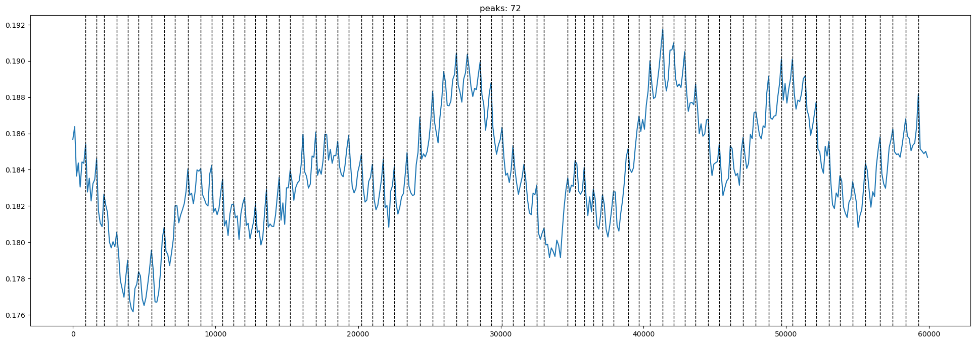
data_type_group: unprocessed rawNow plot the signals with the found peaks from the AMPD for Channel S1D1
[8]:
# select a channel for displaying the results
channel = "S1D1"
channel_data = amp.sel(channel=channel)

# retrieve the peaks for that channel. peaks contains lists for the channel and both wavelengths
# where peaks are represented by 1 and non-peaks are 0
peak_indices = peaks.sel(channel=channel)

# extract the timestamps of the identified peaks for one wavelength
peak_times = times * peak_indices.values[1]
peak_times = [pt for pt in peak_times if pt > 0]

# for plotting prepare the signal for the same wavelength
signal = channel_data.values[1]

# plot the signal and the peaks calculated by the optimized AMPD
plot_peaks(signal, times, peak_times, channel, f"peaks: {len(peak_times)}")
[9]:
cedalion.bib.dump_to_notebook()
Methods used
| [1] | Luke2021 | cedalion.data.get_fingertapping_snirf_path | Robert Luke and David McAlpine. fNIRS Finger Tapping Data in BIDS Format. September 2021. doi:10.5281/zenodo.5529797. |
| [2] | Tucker2022 | cedalion.io.snirf.read_snirf | Stephen Tucker, Jay Dubb, Sreekanth Kura, Alexander von Lühmann, Robert Franke, Jörn M. Horschig, Samuel Powell, Robert Oostenveld, Michael Lührs, Édouard Delaire, Zahra M. Aghajan, Hanseok Yun, Meryem A. Yücel, Qianqian Fang, Theodore J. Huppert, Blaise deB. Frederick, Luca Pollonini, David A. Boas, and Robert Luke. Introduction to the shared near infrared spectroscopy format. Neurophotonics, 10(1):013507, 2022. doi:10.1117/1.NPh.10.1.013507. |
| [3] | Scholkmann2012 | cedalion.sigproc.physio.ampd | Felix Scholkmann, Jens Boss, and Martin Wolf. An efficient algorithm for automatic peak detection in noisy periodic and quasi-periodic signals. Algorithms, 5(4):588–603, 2012. doi:10.3390/a5040588. |